Logistic regression

Inference

Author

Prof. Maria Tackett

Published

Mar 24, 2026

Announcements

Project EDA due TODAY at 11:59pm (on GitHub)
HW 04 due March 31 at 11:59pm
- Released after class
Statistics experience due April 15
SSMU Data Mini #3 - April 4
- See Ed Discussion for full announcement

Topics

Model assessment using ROC curve and AUC
Estimating coefficients for logistic regression model
Inference for a single model coefficient

Computational setup

# load packages
library(tidyverse)
library(tidymodels)
library(openintro)
library(knitr)
library(kableExtra)  # for table embellishments
library(patchwork)

# set default theme and larger font size for ggplot2
ggplot2::theme_set(ggplot2::theme_bw(base_size = 16))

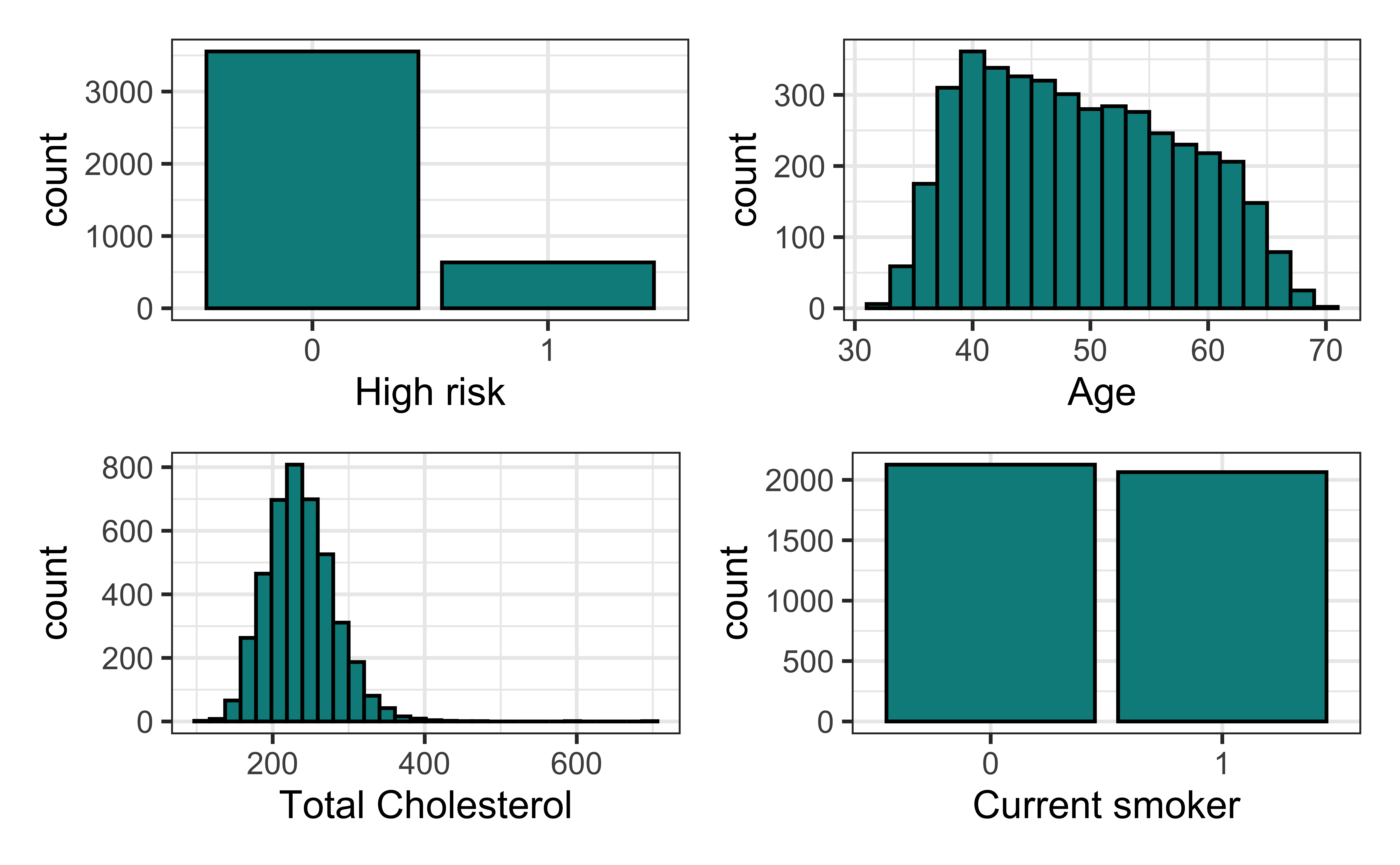
Data: Risk of coronary heart disease

This data set is from an ongoing cardiovascular study on residents of the town of Framingham, Massachusetts.

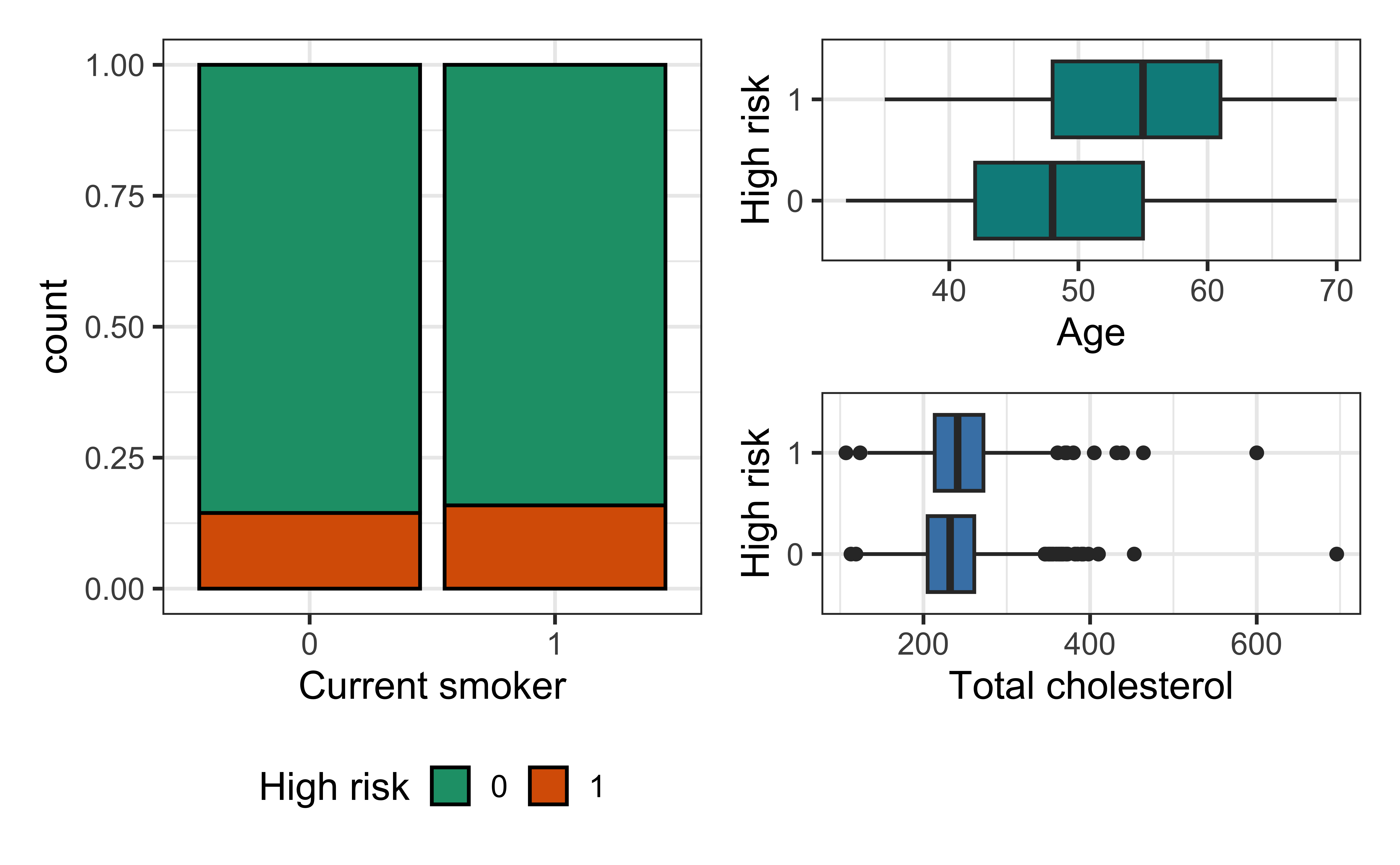
high_risk: 1 = High risk of having heart disease in next 10 years, 0 = Not high risk of having heart disease in next 10 years
age: Age at exam time (in years)
totChol: Total cholesterol (in mg/dL)
currentSmoker: 0 = nonsmoker; 1 = smoker

The goal is to use logistic regression to identify patients who are high risk of heart disease.

Univariate EDA

Bivariate EDA

Risk of coronary heart disease

heart_disease_fit <- glm(high_risk ~ age + totChol + currentSmoker, 
              data = heart_disease, family = "binomial")

term	estimate	std.error	statistic	p.value
(Intercept)	-6.638	0.372	-17.860	0.000
age	0.082	0.006	14.430	0.000
totChol	0.002	0.001	2.001	0.045
currentSmoker1	0.457	0.092	4.951	0.000

ROC curve and AUC

Prediction and classification

We are often interested in using the model to classify observations, i.e., predict whether a given observation will have a 1 or 0 response
For each observation
- Use the logistic regression model to calculate the predicted log-odds the response for the \(i^{th}\) observation is 1
- Use the log-odds to calculate the predicted probability the \(i^{th}\) observation is 1
- Then, use the predicted probability to classify the observation as having a 1 or 0 response using some predefined threshold

Confusion matrix

A confusion matrix is a \(2 \times 2\) table that compares the predicted and actual classes for a given threshold. We can produce this matrix using the conf_mat() function in the yardstick package (part of tidymodels).

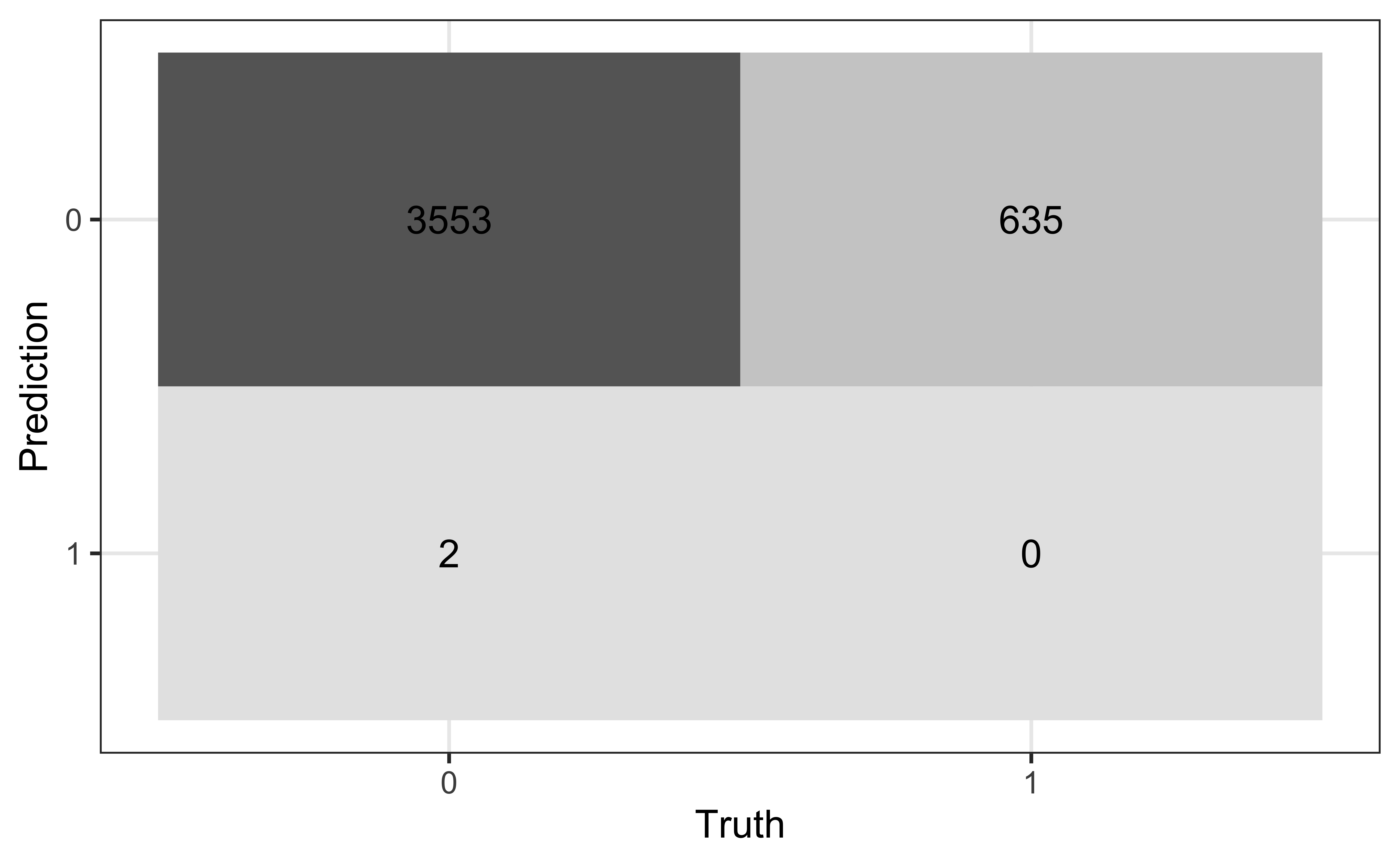
True/false positive/negative

	Not high risk \((y_i = 0)\)	High risk \((y_i = 1)\)
Classified not high risk \((\hat{\pi}_i \leq \text{threshold})\)	True negative (TN)	False negative (FN)
Classified high risk \((\hat{\pi}_i > \text{threshold})\)	False positive (FP)	True positive (TP)

Sensitivity and specificity

How do we set the threshold if the primary goal is high sensitivity?
How do we set the threshold if the primary goal is high specificity?

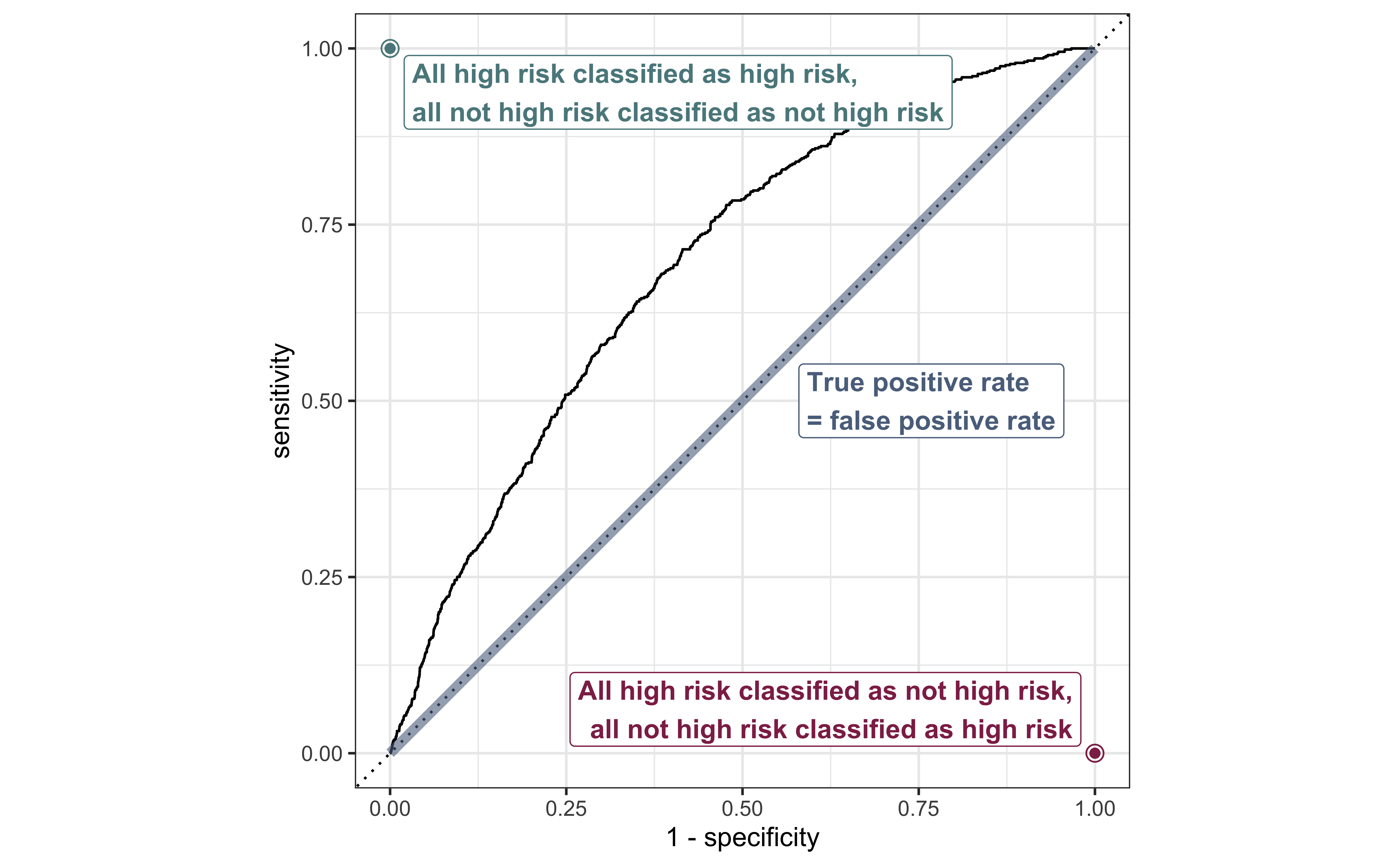
🔗 https://forms.office.com/r/ysNdXsj5cW

ROC Curve

So far the model assessment has depended on the model and selected threshold. The receiver operating characteristic (ROC) curve allows us to assess the model performance across a range of thresholds.

. . .

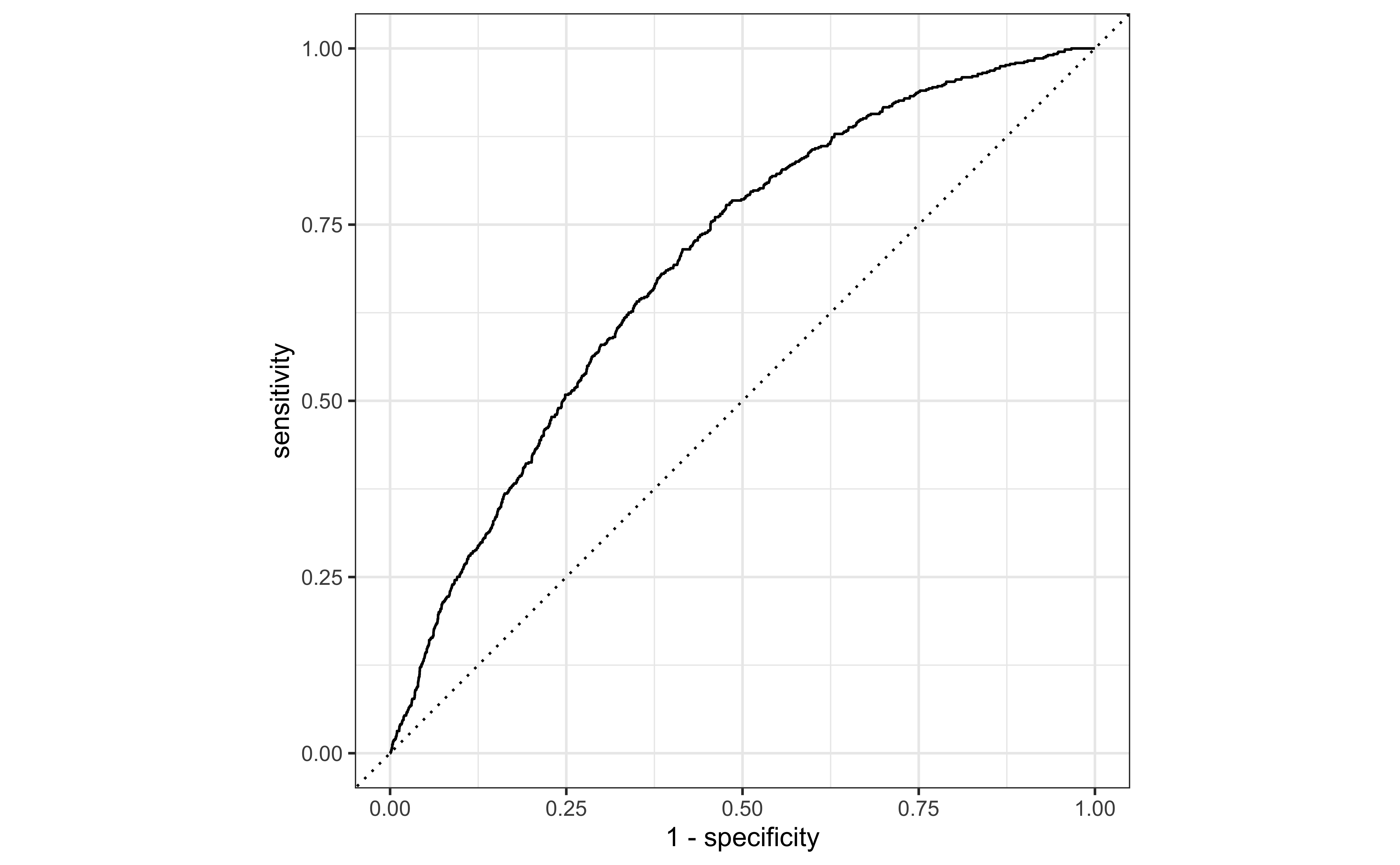
x-axis: 1 - Specificity (False positive rate)
y-axis: Sensitivity (True positive rate)

Which corner of the plot indicates the best model performance?

ROC curve

ROC curve in R

# calculate sensitivity and specificity at each threshold
roc_curve_data <- heart_disease_aug |>
  roc_curve(high_risk, .fitted, 
            event_level = "second") 

# plot roc curve
autoplot(roc_curve_data)

ROC curve in R

Randomly selected observations from roc_data

# A tibble: 20 × 3
   .threshold specificity sensitivity
        <dbl>       <dbl>       <dbl>
 1     0.0778      0.268       0.929 
 2     0.119       0.505       0.784 
 3     0.0990      0.406       0.852 
 4     0.0664      0.185       0.959 
 5     0.354       0.974       0.0614
 6     0.102       0.422       0.839 
 7     0.144       0.610       0.682 
 8     0.225       0.815       0.394 
 9     0.135       0.577       0.715 
10     0.0826      0.302       0.910 
11     0.283       0.922       0.217 
12     0.136       0.581       0.715 
13     0.0659      0.181       0.959 
14     0.298       0.938       0.175 
15     0.0554      0.110       0.980 
16     0.161       0.670       0.614 
17     0.136       0.584       0.715 
18     0.0511      0.0861      0.983 
19     0.111       0.466       0.808 
20     0.0612      0.145       0.969

Area under the curve

The area under the curve (AUC) can be used to assess how well the logistic model fits the data

AUC=0.5: model is a very bad fit (no better than a coin flip)
AUC close to 1: model is a good fit

. . .

heart_disease_aug |>
  roc_auc(high_risk, .fitted,
    event_level = "second"
  )

# A tibble: 1 × 3
  .metric .estimator .estimate
  <chr>   <chr>          <dbl>
1 roc_auc binary         0.696

Estimating coefficients

Statistical model

The form of the statistical model for logistic regression is

\[ \log\Big(\frac{\pi_i}{1-\pi_i}\Big) = \beta_0 + \beta_1x_{i1} + \beta_2x_{i2} + \dots + \beta_px_{ip} \]

where \(\pi_i\) is the probability \(y_i = 1\).

. . .

The response variable \(Y\) follows a Bernoulli distribution, \(\text{Bernoulli}(\pi)\) , so \(E(y_i|x_{i1}, \ldots, x_{ip}) = \pi_i\)

The logit, \(\log\Big(\frac{\pi_i}{1-\pi_i}\Big)\), is called a link function, because it links the expected value to the predictors

Distribution of \(Y\)

The response variable \(Y\) follows a Bernoulli distribution, \(\text{Bernoulli}(\pi)\)

. . .

For an individual observation,

\[ p(y_i | x_{i1}, \ldots, x_{ip}, \beta_0, \beta_1, \ldots, \beta_p) = \pi_i^{y_i}(1 - \pi_i)^{1- y_i} \]

Likelihood function

The likelihood function is the joint density of \(y_1, \ldots, y_n\) for unknown coefficients \(\beta_0, \ldots, \beta_p\)

\[ \begin{aligned} L &= \prod_{i=1}^{n} p(y_i | x_{i1}, \ldots, x_{ip}, \beta_0, \beta_1, \ldots, \beta_p) \\[8pt] & = \prod_{i=1}^{n} \pi_i^{y_i}(1 - \pi_i)^{1- y_i} \end{aligned} \]

. . .

The estimated coefficients are the combination of \(\hat{\beta}_0, \hat{\beta}_1, \ldots, \hat{\beta}_p\) that maximize the likelihood \(L\). They are the maximum likelihood estimates.

Estimating coefficients

We use the log-likelihood function to find the maximum likelihood estimates

\[ \log L = \sum\limits_{i=1}^n[y_i \log(\hat{\pi}_i) + (1 - y_i)\log(1 - \hat{\pi}_i)] \]

where

\(\hat{\pi}_i = \frac{\exp\{\hat{\beta}_0 + \hat{\beta}_1x_{i1} + \dots + \hat{\beta}_px_{ip}\}}{1 + \exp\{\hat{\beta}_0 + \hat{\beta}_1x_{i1} + \dots + \hat{\beta}_px_{ip}\}}\)

Iterative model fitting in R

high_risk_fit_full <- glm(high_risk ~ age + currentSmoker,
                          data = heart_disease, family = "binomial", 
                          # print each iteration
                        control = glm.control(trace = TRUE))

Tracing glm.fit(x = structure(c(1, 1, 1, 1, 1, 1, 1, 1, 1, 1, 1, 1, 1,  .... on entry 
Deviance = 3357.807 Iterations - 1
NULL
Deviance = 3316.428 Iterations - 2
[1] -4.31596973  0.05034933  0.25571505
Deviance = 3315.711 Iterations - 3
[1] -6.03166535  0.08008619  0.42967123
Deviance = 3315.711 Iterations - 4
[1] -6.24973646  0.08351662  0.45215241
Deviance = 3315.711 Iterations - 5
[1] -6.25510967  0.08360203  0.45269557

#stop printing for future models
untrace(glm.fit)

Inference for coefficients

There are two approaches for testing coefficients in logistic regression

(Wald) hypothesis test: Use to test
- a single coefficient (when \(n\) is large)
Drop-in-deviance test: Use to test…
- a single coefficient
- a categorical predictor with 3+ levels
- a group of predictor variables

Hypothesis test for \(\beta_j\)

Hypotheses: \(H_0: \beta_j = 0 \hspace{2mm} \text{ vs } \hspace{2mm} H_a: \beta_j \neq 0\), given the other variables in the model

. . .

(Wald) Test Statistic: \[z = \frac{\hat{\beta}_j - 0}{SE(\hat{\beta}_j)}\]

. . .

P-value: \(P(|Z| > |z|)\), where \(Z \sim N(0, 1)\), the Standard Normal distribution

Coefficient for `age`

Code

high_risk_fit <- glm(high_risk ~ age +  currentSmoker,
                          data = heart_disease, family = "binomial",
                     control = glm.control(trace = FALSE))

tidy(high_risk_fit, conf.int = TRUE) |> 
  kable(digits = 5) |>
  row_spec(2, background = "#D9E3E4")

term	estimate	std.error	statistic	conf.low	conf.high
(Intercept)	-6.25511	0.31504	-19.85519	-6.88001	-5.64472
age	0.08360	0.00556	15.04622	0.07279	0.09458
currentSmoker1	0.45270	0.09227	4.90642	0.27230	0.63410

. . .

Hypotheses:

\[ H_0: \beta_{age} = 0 \hspace{2mm} \text{ vs } \hspace{2mm} H_a: \beta_{age} \neq 0 \], given current smoking status is in the model

Coefficient for `age`

term	estimate	std.error	statistic	conf.low	conf.high
(Intercept)	-6.25511	0.31504	-19.85519	-6.88001	-5.64472
age	0.08360	0.00556	15.04622	0.07279	0.09458
currentSmoker1	0.45270	0.09227	4.90642	0.27230	0.63410

Test statistic:

\[z = \frac{0.08360 - 0}{0.00556} = 15.04 \]

Coefficient for `age`

term	estimate	std.error	statistic	conf.low	conf.high
(Intercept)	-6.25511	0.31504	-19.85519	-6.88001	-5.64472
age	0.08360	0.00556	15.04622	0.07279	0.09458
currentSmoker1	0.45270	0.09227	4.90642	0.27230	0.63410

P-value:

\[ P(|Z| > |15.04|) \approx 0 \]

. . .

2 * pnorm(15.04,lower.tail = FALSE)

[1] 4.015501e-51

Coefficient for `age`

term	estimate	std.error	statistic	conf.low	conf.high
(Intercept)	-6.25511	0.31504	-19.85519	-6.88001	-5.64472
age	0.08360	0.00556	15.04622	0.07279	0.09458
currentSmoker1	0.45270	0.09227	4.90642	0.27230	0.63410

Conclusion:

The p-value is very small, so we reject \(H_0\). The data provide sufficient evidence that age is a statistically significant predictor of whether someone is high risk of having heart disease, after accounting for smoking status.

Confidence interval for \(\beta_j\)

We compute the C% confidence interval for \(\beta_j\) as the following:

\[ \hat{\beta}_j \pm z^* \times SE_{\hat{\beta}_j} \]

where \(z^*\) is the critical value from the \(N(0,1)\) distribution

# z* for 95% confidence interval 
qnorm(0.975, mean = 0, sd = 1)

[1] 1.959964

. . .

Note

This is an interval for the change in the log-odds for every one unit increase in \(x_j\)

Interpretation in terms of the odds

The change in odds for every one unit increase in \(x_j\).

\[ \exp\{\hat{\beta}_j \pm z^* \times SE_{\hat{\beta}_j}\} \]

. . .

Interpretation: We are \(C\%\) confident that for every one unit increase in \(x_j\), the odds multiply by a factor of \(\exp\{\hat{\beta}_j - z^*\times SE_{\hat{\beta}_j}\}\) to \(\exp\{\hat{\beta}_j + z^* \times SE_{\hat{\beta}_j}\}\), holding all else constant.

CI for `age`

term	estimate	std.error	statistic	conf.low	conf.high
(Intercept)	-6.255	0.315	-19.855	-6.880	-5.645
age	0.084	0.006	15.046	0.073	0.095
currentSmoker1	0.453	0.092	4.906	0.272	0.634

Interpret the 95% confidence interval for age in terms of the odds of being high risk for heart disease.

Recap

Model assessment using ROC curve and AUC
Estimating coefficients for logistic regression model
Inference for a single model coefficient

Next class

Model selection for logistic regression
Complete Lecture 19 prepare

Announcements

Topics

Computational setup

Data: Risk of coronary heart disease

Univariate EDA

Bivariate EDA

Risk of coronary heart disease

ROC curve and AUC

Prediction and classification

Confusion matrix

True/false positive/negative

Sensitivity and specificity

ROC Curve

ROC curve

ROC curve in R

ROC curve in R

Area under the curve

Estimating coefficients

Statistical model

Distribution of \(Y\)

Likelihood function

Estimating coefficients

Iterative model fitting in R

Inference for coefficients

Inference for coefficients

Hypothesis test for \(\beta_j\)

Coefficient for age

Coefficient for age

Coefficient for age

Coefficient for age

Confidence interval for \(\beta_j\)

Interpretation in terms of the odds

CI for age

Recap

Next class

Coefficient for `age`

Coefficient for `age`

Coefficient for `age`

Coefficient for `age`

CI for `age`