library(tidyverse)  # for data wrangling
library(tidymodels) # for modeling and inference
library(knitr)      # to neatly format tables
library(sf)         # for working with spatial data
library(tigris)     # for shape files of US counties

# load other packages as needed HW 01: Simple linear regression
Cost of preschool in the United States
Important
This assignment is due on Tuesday, January 27 at 11:59pm. To be considered on time, the following must be done by the due date:
Final
.qmdand.pdffiles pushed to your GitHub repoFinal
.pdffile submitted on Gradescope
Introduction
In this assignment, you will use simple linear regression to examine the association between median income and the median weekly cost of preschool in the United States.
Learning goals
In this assignment, you will…
fit and interpret simple linear regression models.
construct and interpret bootstrap confidence intervals for the population slope, \(\beta_1\).
describe visualizations highlight different features of a distribution.
continue developing a workflow for reproducible data analysis.
Getting started
Go to the sta210-sp26 organization on GitHub. Click on the repo with the prefix hw-01. It contains the starter documents you need to complete the lab.
Clone the repo and start a new project in RStudio. See the Lab 00 for details on cloning a repo and starting a new project in R.
The following packages will be used in this assignment:
Data: Counties in the United States
The dataset in this assignment includes demographic, socioeconomic, and childcare cost information for 600 randomly selected counties in the United States (about 19% of all counties). The data are originally from the National Database of Childcare Prices and were featured as part of the TidyTuesday weekly data visualization challenge in May 2023.
The data are in the file childcare-2018-sample.csv located in the data folder of your GitHub repo. This analysis focuses on the following variables:
me_2018: Median income in 2018 for the population aged 16 years old or older.mc_preschool: Aggregated weekly, full-time median price charged for Center-based Care for preschoolers (i.e. aged 36 through 54 months) in 2018
Click here for the full codebook for the TidyTuesday data set.
childcare <- read_csv("data/childcare-2018-sample.csv") Exercises
The goal of this analysis is to explore the relationship between individuals’ annual income and the cost of preschool in a county. More specifically, we wish to describe how much the cost of preschool typically changes as the income in a county increase.
ImportantInstructions
Type your responses to each question in your Quarto document. Write all narrative using complete sentences and include informative axis labels and titles on visualizations. Use a reproducible workflow by periodically rendering the Quarto document, writing an informative commit message, and pushing the updated .qmd and .pdf files to GitHub.
Part 1: Exploratory data analysis
Exercise 1
Create a histogram of the distribution of the response variable mc_preschool and compute the summary statistics. Use the visualization and summary statistics to describe the distribution. Include an informative title and axis labels on the plot.
Tip
The description should include shape, center, spread, and presence of outliers. Use specific values in your description. See Section 3.4.2 of Introduction to Regression Analysis for more information about describing univariate distributions. See the ggplot2 reference for example code and plots.
Exercise 2
Let’s view the data in another way. Below is a map showing the 600 counties in our sample filled in based on values of mc_preschool. The code for the map was adapted from code produced by ChatGPT (model GPT-5.2).
What are 2 observations you have from the map?
What is a feature that is apparent in the map that wasn’t as easily apparent from the histogram in the previous exercise? What is a feature that is apparent in the histogram that is not as easily apparent from the map?
Code
map_data_sample <-  read_csv("data/county-map-2018.csv")

# create data frame containing mapping data for all counties
counties_sf <- counties(cb = TRUE, year = 2018) |>
  st_as_sf() |>
  mutate(fips = paste0(STATEFP, COUNTYFP))

# join mapping data to analysis data
county_map_data <- counties_sf |>
  left_join(childcare, by = "fips")

# produce map
county_map <- ggplot(county_map_data) +
  geom_sf(aes(fill = mc_preschool), color = NA) +
  scale_fill_viridis_c(na.value = "grey90") +
  coord_sf(
    xlim = c(-125, -66),
    ylim = c(24, 50),
    expand = FALSE)  +
  labs(title = "Median weekly preschool costs",
       subtitle = "for 600 counties in the United States",
       fill = "Median cost") +
theme_void() 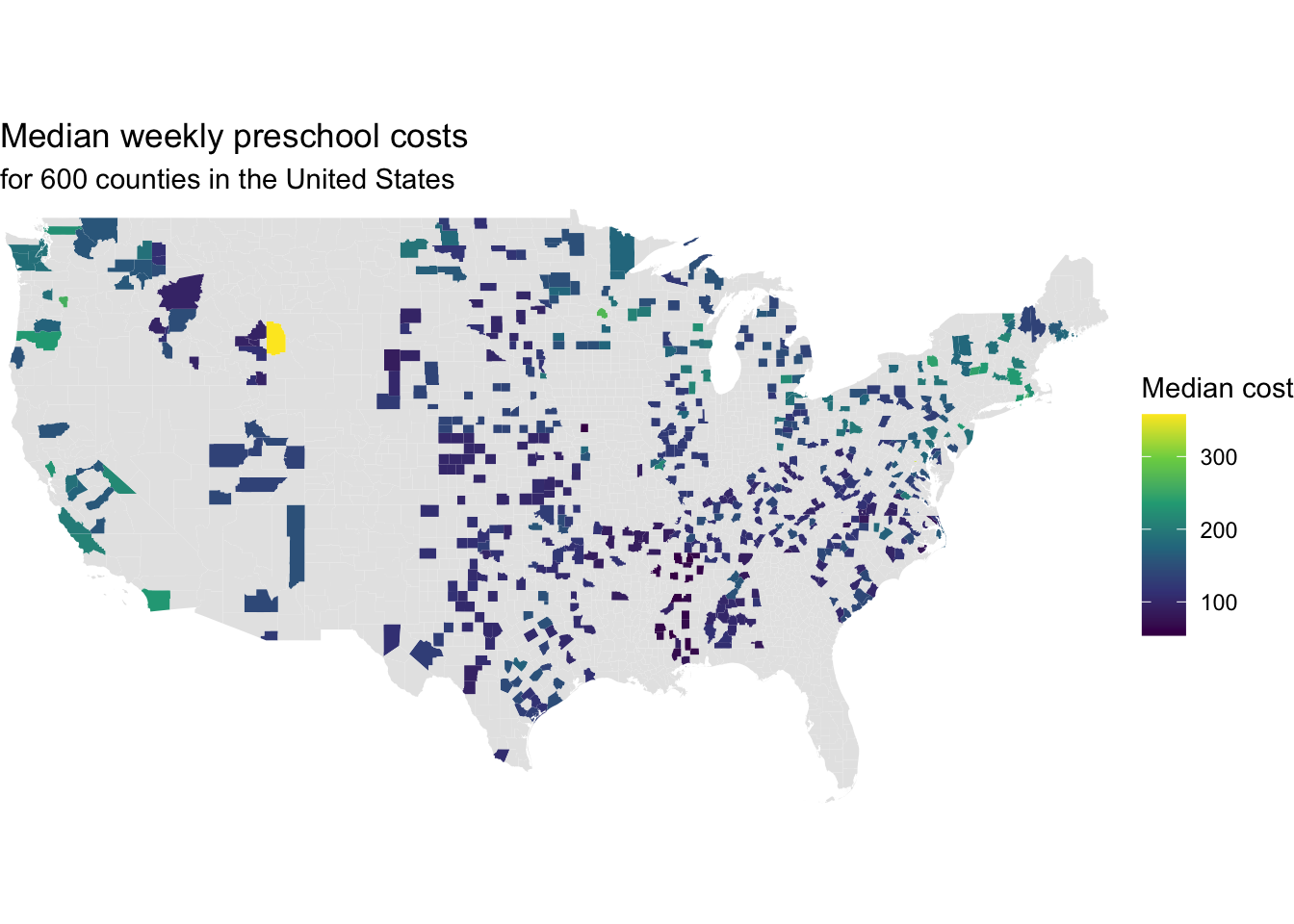
Exercise 3
Create a visualization of the relationship between me_2018 and mc_preschool (originally said mc_toddler) and compute the correlation. Use the visualization and correlation to describe the relationship between the two variables.
This is a good place to render, commit, and push changes to your hw-01 repo on GitHub. Write an informative commit message (e.g. “Completed exercises 1 - 3”), and push every file to GitHub by clicking the check box next to each file in the Git pane. After you push the changes, the Git pane in RStudio should be empty.
Part 2: Modeling
Exercise 4
We will use a linear regression model to explain variability in mc_preschool based on me_2018.
Write the form of the statistical (theoretical) model using mathematical notation. In your response, make it clear which variable (me_2018 or mc_preschool) is the predictor and which variable is the response.
Tip
Use the following code format to make the variable names properly render in the PDF document.
\(\text{me\_2018}\) = \text{me\_2018}
\(\text{mc\_preschool}\) = \text{mc\_preschool}
Exercise 5
Fit the regression line corresponding to the statistical model in the previous exercise. Neatly display the model output using 3 digits.
Write the equation of the fitted model using mathematical notation. In your response, make it clear which variable (
me_2018ormc_preschool) is the predictor and which variable is the response.
Exercise 6
Interpret the slope in the context of the data.
Does the intercept have a meaningful interpretation? If so, write the interpretation in the context of the data. Otherwise, briefly explain why not.
Exercise 7
- In 2018, the median income in Durham County was $35,436. What is the predicted median weekly cost for preschool based on the model in Exercise 5?
- The actual median cost for preschool was $173 per week. What is the residual?
This is a good place to render, commit, and push changes to your hw-01 repo on GitHub. Write an informative commit message (e.g. “Completed exercises 4 -7”), and push every file to GitHub by clicking the check box next to each file in the Git pane. After you push the changes, the Git pane in RStudio should be empty.
Part 3: Inference
We will use the data from these 600 randomly selected counties to draw conclusions about the relationship between income and weekly cost of preschool for the over 3,000 counties in the United States.
Exercise 8
What is the population in this analysis? What is the sample?
Is it reasonable to treat the sample in this analysis as representative of the population? Briefly explain why or why not.
Exercise 9
Construct a 90% bootstrap confidence interval for the slope. Use set.seed(2026) and 1000 iterations. Show all relevant code and output used to produce the interval.
Write the 90% confidence interval using 3 digits.
Exercise 10
Interpret the interval from the previous exercise in the context of the data.
You want to use the confidence interval to evaluate the claim that there is no linear relationship between median income and cost of preschool. In other words, you want to evaluate the claim that \(\beta_1 = 0\) in the model written in Exercise 4.
Does the confidence interval from the previous exercise support this claim? Briefly explain why or why not.
Now is a good time to render your document again if you haven’t done so recently, commit (with an informative commit message), and push all updates.
AI Disclosure
Did you use an LLM / Generative AI tool to complete this assignment? If not, copy and paste the first option in your Quarto document. Otherwise, copy and paste all statements that describe how you used it. The purpose of the disclosure is for you to reflect on how you’re using AI in this course. It also helps learn how students are most effectively using AI.
- I didn’t an LLM / Generative AI tool.
- I asked it to clarify one or more exercises.
- I asked it clarifying questions to better understand a concept.
- I asked it to help write code to complete an exercise.
- I gave it my code and asked it to help me fix it.
- I asked it about an error or why code would do something I didn’t want.
- I pasted the exercise prompt in AI and asked for help, but I wrote my answer myself.
- I pasted the exercise prompt in AI and copied and pasted at least some of the answer into my Quarto document.
- Other:______
Submission
Warning
Before you wrap up the assignment, make sure all documents are updated on your GitHub repo. We will be checking these to make sure you have been practicing how to commit and push changes.
Remember – you must turn in a PDF file to the Gradescope page before the submission deadline for full credit.
To submit your assignment:
Access Gradescope through the STA 210 Canvas site.
Click on the assignment, and you’ll be prompted to submit it.
Mark the pages associated with each exercise. All of the pages of your lab should be associated with at least one question (i.e., should be “checked”).
Select the first page of your .PDF submission to be associated with the “Workflow & formatting” section.
Grading (50 points)
| Component | Points |
|---|---|
| Ex 1 | 5 |
| Ex 2 | 4 |
| Ex 3 | 5 |
| Ex 4 | 4 |
| Ex 5 | 5 |
| Ex 6 | 5 |
| Ex 7 | 4 |
| Ex 8 | 4 |
| Ex 9 | 6 |
| Ex 10 | 4 |
| Completing AI Disclosure | 1 |
| Workflow & formatting | 3 |
The “Workflow & formatting” grade is to assess the reproducible workflow and document format for the applied exercises. This includes having at least 3 informative commit messages, a neatly organized document with readable code and your name and the date updated in the YAML.