This page contains practice problems to help prepare for Exam 01. This set of practice problems is not comprehensive.
There is no answer key for these problems. You are encouraged to ask questions during office hours or on Ed Discussion.
Data
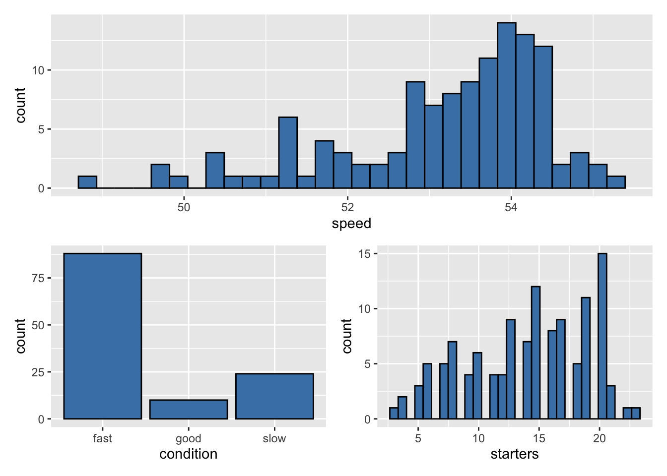
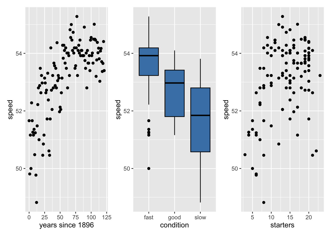
We will review data about the Kentucky Derby, an annual 1.25-mile horse race held at the Churchill Downs race track in Louisville, Kentucky. The variables are the following:
years_since_1896: Number of years since 1896 (the first year of data in our data set)
winner: The winning horse
condition : Condition of the track (fast, good, slow)
speed: average speed of the winner (in feet per second)
Interpret the coefficient of years_since_1896 in the context of the data.
What is the baseline category for condition?
Interpret the coefficient of conditiongood in the context of the data.
Exercise 3
Does the intercept have a meaningful interpretation?
If not, what are some strategies we can use to fit a model in which the intercept is meaningful?
Exercise 4
There are three conditions in the data set (fast, good, slow), but only two terms for condition in the model. Conceptually explain why we cannot put indicators for all three conditions along with the intercept in the model.
Exercise 5
We want to test whether there is evidence that the winners are getting faster over time. To do so, we conduct the following hypothesis test for the coefficient of years_since_1896.
Null: There is no linear relationship between years_since_1896 and speed, after accounting condition and starters
Alternative: There is no linear relationship between years_since_1896 and speed, after accounting condition and starters
Write these hypotheses in mathematical notation.
The standard error is 0.002. Explain what this value means in the context of the data.
The test statistic is 9.766. Explain how this value is computed and what this value means in the context of the data.
What distribution is used to compute the p-value? Be specific.
What is the conclusion from the test in the context of the data?
Does this hypothesis test answer the stated analysis question?
Exercise 6
Interpret the 95% confidence interval for years_since_1896 in the context of the data.
Is the interval consistent with the test from the previous exercise? Briefly explain.
Exercise 7
Describe the effect of the track condition on the average speed of the winner. In the description, include discussion of the estimated coefficients along with the results from statistical inference.
Exercise 8
We want to consider a potential interaction effect between starters and condition. Sketch a scatterplot that shows the relationship between starters and speed differing by condition.
Exercise 9
The output of the model that includes the interaction between starters and conditions is shown below:
Interpret the coefficient of conditiongood:starters in the context fo the data.
Write the estimated model for fast track conditions.
What is the effect of starters went the track condition is slow?
Exercise 10
We conduct inference on the coefficients \(\beta_j\) assuming that the variability of \(Y|X_1, \ldots, X_p\) is equal for all values (or combination of values) of the predictor(s). Briefly explain why this assumption is important.
Exercise 11
Explain why we say “holding all else constant” when interpreting the coefficients in a multiple linear regression model.
Exercise 12
Suppose we construct a bootstrap confidence interval for \(\beta_{\text{starters}}\). We use 1,000 iterations and the seed 210
What is the approximate center of the bootstrap distribution?
How many observations are in the bootstrap sample for a single iteration?
What is the approximate variance of the bootstrap distribution?
Exercise 13
Describe how indicator variables, if at all, impact a model (e.g., the intercept, the slope, both).
Describe how interaction terms, if at all, impact a model (e.g., the intercept, the slope, both).
Exercise 14
Explain why the equal variance condition is important for inference based on mathematical models but not important for simulation-based inference.
Relevant lectures, assignments and AEs
Ask yourself “why” questions as you review the slides, along with your answers and problem-solving process on the lectures and assignments. It can also be helpful to explain your process to others.
Lectures: January 8 - February 12 (February 12 lecture is an exam review)