library(tidyverse)
library(tidymodels)
library(knitr)
library(patchwork)

# add other packages as neededLab 04: Exam 01 Review
ImportantDue date
Turn in what you have at the end of your lab section on February 16 for credit on the lab. To be considered on time, the following must be done by the due date:
- Final
.qmdand.pdffiles pushed to your team’s GitHub repo - Final
.pdffile submitted on Gradescope
Getting started
Go to the sta210-sp26 organization on GitHub. Click on the repo with the prefix lab-04-. It contains the starter documents you need to complete the lab.
Clone the repo and start a new project in RStudio. See the Lab 00 instructions for details on cloning a repo, starting a new project in R, and configuring git.
Packages
You will need the following packages for the lab:
Restaurant tips
What factors are associated with the amount customers tip at a restaurant? To answer this question, we will use data collected in 2011 by a student at St. Olaf who worked at a local restaurant.1
The variables we’ll focus on for this analysis are
Tip: amount of the tipParty: number of people in the partyAge: Age of the payer
View the data set to see the remaining variables.
tips <- read_csv("data/tip-data.csv")Exploratory data analysis
Code
p1 <- ggplot(data = tips, aes(x = Tip)) +
  geom_histogram(color = "white", binwidth = 2) +
  labs(x = "Tips ($)",
       title = "Tips at local restaurant")

p2 <- ggplot(data = tips, aes(x = Party)) +
  geom_histogram(color = "white") +
  labs(x = "Party",
       title = "Number of diners in party") +
  xlim(c(0, 7))

p3 <- ggplot(data = tips, aes(x = Age)) +
  geom_bar(color = "white") +
  labs(x = "",
       title = "Age of Payer")

p1 / (p2 + p3)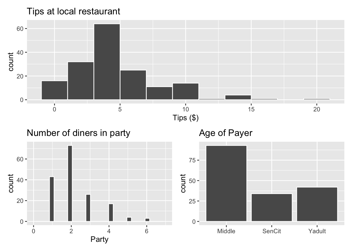
Code
p4 <- ggplot(data = tips, aes(x = Party, y = Tip)) +
  geom_jitter() +
  labs(x = "Number of diners in party",
       y = "Tips ($)",
       title = "Tips vs. Party")

p5 <- ggplot(data = tips, aes(x = Age, y = Tip)) +
  geom_boxplot() +
  labs(x = "Age of payer",
       y = "Tips ($)",
       title = "Tips vs. Age")

p4 + p5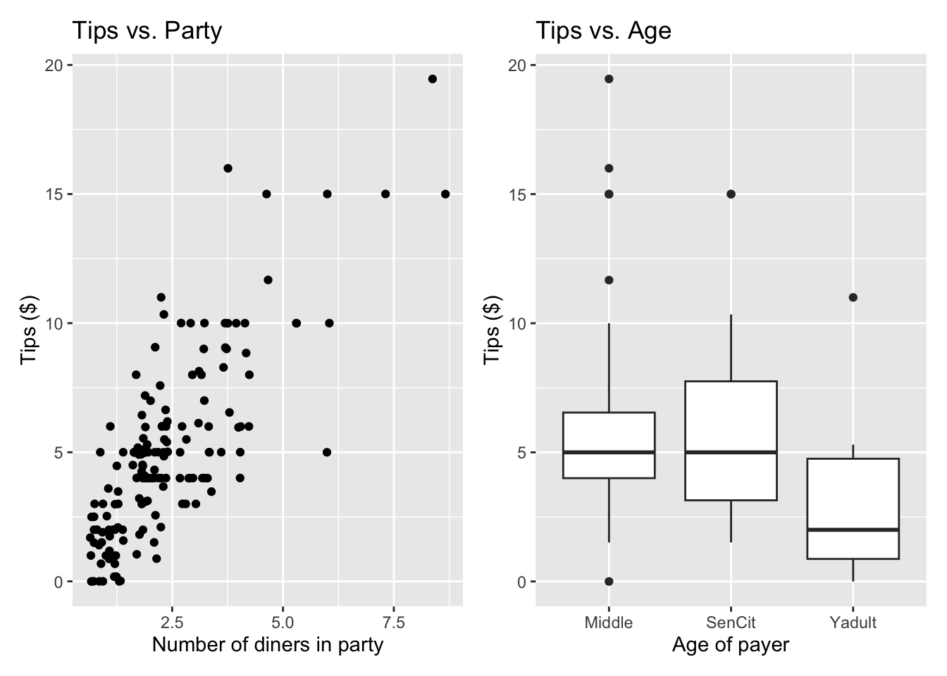
We will use the number of diners in the party and age of the payer to understand variability in the tips.
Exercise 1
We will start with the main effects model that includes Age and Party.
Fit the model and neatly display the results with 95% confidence intervals for the coefficients, using 2 decimal places.
Interpret the coefficient of
Partyin the context of the data.Compute the regression standard error \(\hat{\sigma}_\epsilon\) and interpret this value in the context of the data.
Exercise 2
You wish to use the model in Exercise 1 to test whether there is a linear relationship between tips and the number of diners in the party, after adjusting for the age of the payer. Explain what the test statistic means in the context of the data.
Explain what the p-value means in the context of the data.
State the conclusion from the test in the context of the data.
An article claims that one can expect about $2 in tips for each additional person at a table. Does the model support this claim? Why or why not.
Exercise 3
Let’s check the model conditions for the model from Exercise 1. Below are plots of residuals versus fitted values and the distribution of residuals.
For each model condition (linearity, independence, normality, equal variance), comment on whether the condition is satisfied and briefly explain your response.
Code
tip_model <- lm(Tip ~ Age + Party, data = tips)

tip_model_aug <- augment(tip_model)

resid_fitted <- ggplot(data = tip_model_aug, aes(x = .fitted, y = .resid)) +
  geom_point() +
  geom_hline(yintercept = 0, linetype = 2, color = "red") +
  labs(x = "Fitted values",
       y = "Residuals",
       title = "Residuals versus fitted values")

dist_resid <- ggplot(data = tip_model_aug, aes( x= .resid)) +
  geom_histogram() +
  labs(x = "Residuals",
       title = "Distribution of residuals")

resid_fitted + dist_resid
Exercise 4
One observation in the data set has a leverage of 0.190, standardized residual of -1.499, and Cook’s distance of 0.134. Use these values to comment on the following:
whether the observation has large leverage.
whether the observation has an outlying residual.
whether the observation is an influential point.
Exercise 5
Now let’s fit a model using Age, Party and the interaction between the two variables. Display the 95% confidence interval for the coefficients.
State what the standard error for the coefficient of
AgeSenCit:Partymeans in the context of the data.Write code to show how the 95% confidence interval for
AgeSenCit:Partywas computed.Based on the confidence interval, is there evidence that senior citizens pay less per additional person in the party compared to middle aged diners? Briefly explain.
Exercise 6
We want to consider a new variable other_diners = Party - 1 that is the number of people in the party aside from the payer. We will use this variable in a model that includes Age, other_diners, and the interaction between the two variables.
- What is an advantage to using
other_dinersinstead ofPartyin the model? - How will the responses to the previous exercise change, if at all, by using
other_dinersinstead ofPartyin the model?
Submission
Warning
Before you wrap up the assignment, make sure all documents are updated on your GitHub repo. We will be checking these to make sure you have been practicing how to commit and push changes.
Reminder: you must turn in a PDF file to the Gradescope page before the submission deadline for full credit.
To submit the assignment:
Access Gradescope through the STA 210 Canvas site.
Click on the assignment, and you’ll be prompted to submit it.
Mark the pages for the “Exercises” question.
Grading (10 points)
| Component | Points |
|---|---|
| Submitted by the end of lab | 10 |
Footnotes
Dahlquist, Samantha, and Jin Dong. 2011. “The Effects of Credit Cards on Tipping.” Project for Statistics 212-Statistics for the Sciences, St. Olaf College.↩︎