Logistic regression

Model selection

Author

Prof. Maria Tackett

Published

Mar 26, 2026

Announcements

Lab 06 due TODAY at 11:59pm
HW 04 due March 31 at 11:59pm
Statistics experience due April 15
SSMU Data Mini #3 - April 4
- See Ed Discussion for full announcement

Computational setup

# load packages
library(tidyverse)
library(tidymodels)
library(openintro)
library(knitr)
library(kableExtra)  # for table embellishments
library(Stat2Data)   # for empirical logit

# set default theme and larger font size for ggplot2
ggplot2::theme_set(ggplot2::theme_bw(base_size = 20))

Review from HW 03

Recall the four candidate models for Buchanan vs. Bush in HW 03:

Model	Response variable	Predictor variable	RMSE
1	Buchanan2000	Bush2000	348.6
2	log(Buchanan2000)	Bush2000	0.758
3	Buchanan2000	log(Bush2000)	369.533
4	log(Buchanan2000)	log(Bush2000)	0.460

Why is it unreliable to use these values of RMSE to choose the best fit model?

Topics

Comparing logistic regression models using
- Drop-in-deviance test
- AIC
- BIC
Cross validation for logistic regression

Data: Risk of coronary heart disease

This data set is from an ongoing cardiovascular study on residents of the town of Framingham, Massachusetts. We want to examine the relationship between various health characteristics and the risk of having heart disease.

high_risk:
- 1: High risk of having heart disease in next 10 years
- 0: Not high risk of having heart disease in next 10 years
age: Age at exam time (in years)
education: 1 = Some High School, 2 = High School or GED, 3 = Some College or Vocational School, 4 = College
currentSmoker: 0 = nonsmoker, 1 = smoker
totChol: Total cholesterol (in mg/dL)

Data

# A tibble: 4,086 × 6
     age education TenYearCHD totChol currentSmoker high_risk
   <dbl> <fct>          <dbl>   <dbl> <fct>         <fct>    
 1    39 4                  0     195 0             0        
 2    46 2                  0     250 0             0        
 3    48 1                  0     245 1             0        
 4    61 3                  1     225 1             1        
 5    46 3                  0     285 1             0        
 6    43 2                  0     228 0             0        
 7    63 1                  1     205 0             1        
 8    45 2                  0     313 1             0        
 9    52 1                  0     260 0             0        
10    43 1                  0     225 1             0        
# ℹ 4,076 more rows

Modeling risk of coronary heart disease

Using age, totChol, and currentSmoker

term	estimate	std.error	statistic	p.value	conf.low	conf.high
(Intercept)	-6.673	0.378	-17.647	0.000	-7.423	-5.940
age	0.082	0.006	14.344	0.000	0.071	0.094
totChol	0.002	0.001	1.940	0.052	0.000	0.004
currentSmoker1	0.443	0.094	4.733	0.000	0.260	0.627

Review: ROC Curve + Model fit

high_risk_aug <- augment(high_risk_fit)

roc_curve_data <- high_risk_aug |>
  roc_curve(high_risk, .fitted, event_level = "second")

#calculate AUC
high_risk_aug |>
  roc_auc(high_risk, .fitted, event_level = "second")

# A tibble: 1 × 3
  .metric .estimator .estimate
  <chr>   <chr>          <dbl>
1 roc_auc binary         0.697

Inference for coefficients

There are two approaches for testing coefficients in logistic regression

(Wald) hypothesis test: Use to test
- a single coefficient (when \(n\) is large)
Drop-in-deviance test: Use to test…
- a single coefficient
- a categorical predictor with 3+ levels
- a group of predictor variables

Drop-in-deviance test

Which model do we choose?

Model 1

term	estimate
(Intercept)	-6.673
age	0.082
totChol	0.002
currentSmoker1	0.443

Model 2

term	estimate
(Intercept)	-6.456
age	0.080
totChol	0.002
currentSmoker1	0.445
education2	-0.270
education3	-0.232
education4	-0.035

Log likelihood

\[ \begin{aligned} \log L = \sum\limits_{i=1}^n[y_i \log(\hat{\pi}_i) + (1 - y_i)\log(1 - \hat{\pi}_i)] \end{aligned} \]

. . .

Measure of how well the model fits the data
Higher values of \(\log L\) are better
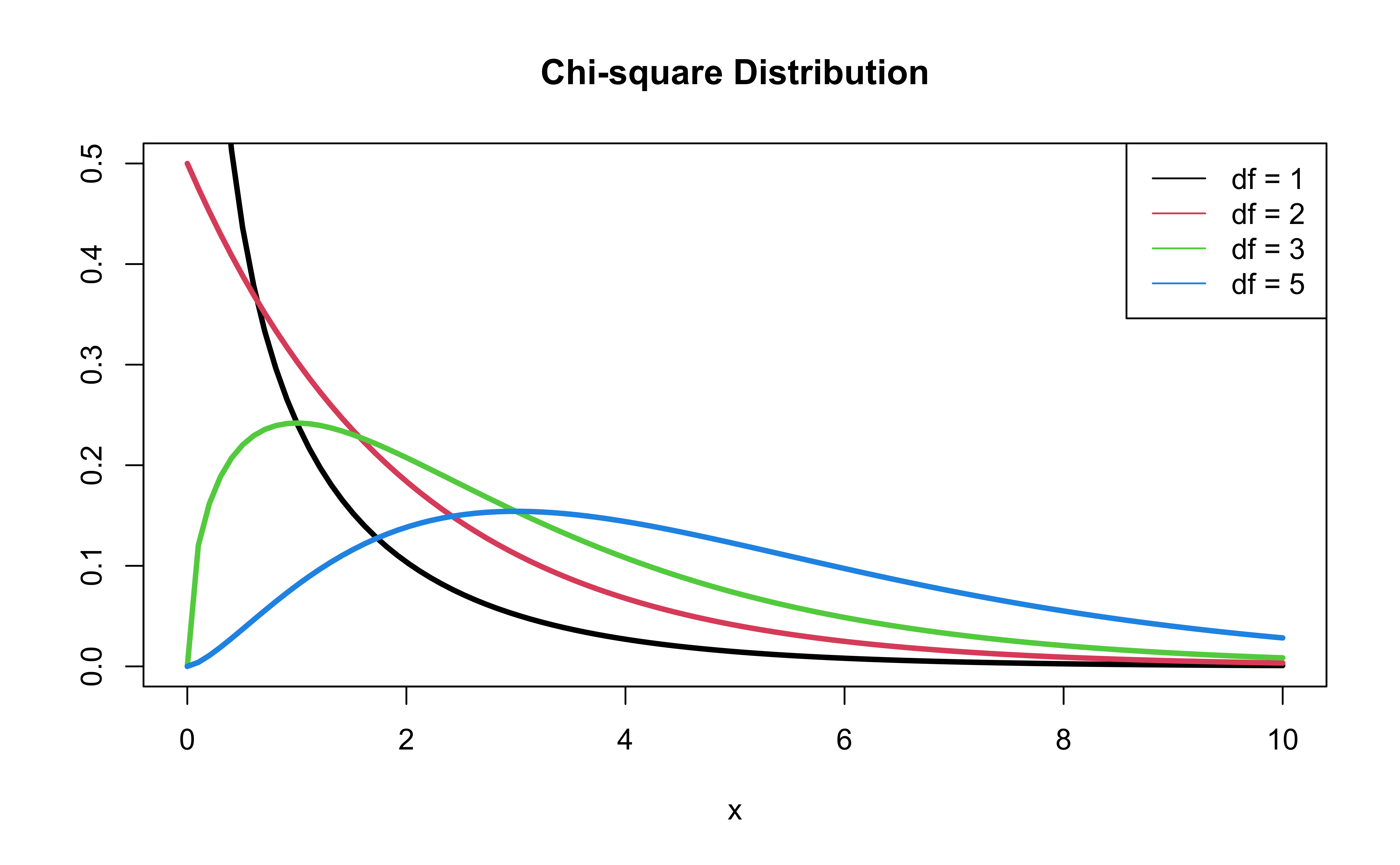
Deviance = \(-2 \log L\)
- \(-2 \log L\) follows a \(\chi^2\) (“Chi squared”) distribution with \(n - p - 1\) degrees of freedom

Comparing nested models

Suppose there are two nested models:
- Reduced Model includes predictors \(x_1, \ldots, x_q\)
- Full Model includes predictors \(x_1, \ldots, x_q, x_{q+1}, \ldots, x_p\)
We want to test the hypotheses

\[ \begin{aligned} H_0&: \beta_{q+1} = \dots = \beta_p = 0 \\ H_a&: \text{ at least one }\beta_j \text{ is not } 0 \end{aligned} \]
To do so, we will use the Drop-in-deviance test, also known as the Nested Likelihood Ratio test

Drop-in-deviance test

Hypotheses:

\[ \begin{aligned} H_0&: \beta_{q+1} = \dots = \beta_p = 0 \\ H_a&: \text{ at least one }\beta_j \text{ is not } 0 \end{aligned} \]

. . .

Test Statistic: \[\begin{aligned}G &= \text{Deviance}_{reduced} - \text{Deviance}_{full} \\ &= (-2 \log L_{reduced}) - (-2 \log L_{full})\end{aligned}\]

. . .

P-value: \(P(\chi^2 > G)\), calculated using a \(\chi^2\) distribution with degrees of freedom equal to the number of parameters being tested

\(\chi^2\) distribution

Add `education` to the model?

Reduced model

high_risk_fit_reduced <- glm(high_risk ~ age + totChol + currentSmoker,
                             data = heart_disease, family = "binomial")

. . .

Full model

high_risk_fit_full <- glm(high_risk ~ age + totChol +
                            currentSmoker + education, 
              data = heart_disease, family = "binomial")

Write the null and alternative hypotheses in words and mathematical notation.

Add `education` to the model?

Compute the deviance for each model:

(dev_reduced <- glance(high_risk_fit_reduced)$deviance)

[1] 3224.812

(dev_full <- glance(high_risk_fit_full)$deviance)

[1] 3217.6

. . .

Drop-in-deviance test statistic:

(test_stat <- dev_reduced - dev_full)

[1] 7.212113

Add `education` to the model?

Calculate the p-value using a pchisq(), with degrees of freedom equal to the number of new model terms in the second model:

pchisq(test_stat, 3, lower.tail = FALSE)

[1] 0.06543567

Add `education` to the model?

The p-value is 0.065. What is your conclusion?

🔗 https://forms.office.com/r/DxiwzbjGvs

Drop-in-Deviance test in R

Use anova() to conduct the drop-in deviance test

Add argument test = "Chisq" to conduct the drop-in-deviance test

. . .

anova(high_risk_fit_reduced, high_risk_fit_full, test = "Chisq") |>
  tidy() |> kable(digits = 3)

term	df.residual	residual.deviance	df	deviance	p.value
high_risk ~ age + totChol + currentSmoker	4082	3224.812	NA	NA	NA
high_risk ~ age + totChol + currentSmoker + education	4079	3217.600	3	7.212	0.065

Applies to linear regression

We can use the drop-in-deviance test to test for subset of predictors in linear regression
The deviance for the linear regression model is the sum of squared residuals

\[ SSR = \sum_{i=1}^n(y_i - \hat{y}_i)^2 \]
The test statistic for the drop-in-deviance test is \[G = SSR_{\text{reduced}} - SSR_{full}\]
This is also called the Nested F Test

Model selection using AIC and BIC

AIC & BIC

Estimators of prediction error and relative quality of models:

. . .

Akaike’s Information Criterion (AIC)¹: \[AIC = -2\log L + 2(p+1)\]

. . .

Bayesian Information Criterion (BIC)²: \[ BIC = -2\log L + \log(n)\times(p+1)\]

AIC & BIC

\[ \begin{aligned} & AIC = -2\log L \color{black}{+ 2(p+1)} \\ & BIC = -2\log L + \color{black}{\log(n)\times(p+1)} \end{aligned} \]

where \(\log L\) is the log-likelihood evaluated at the maximum likelihood estimate, \((p+1)\) is the number of terms in the model, and \(n\) is the sample size

AIC & BIC

\[ \begin{aligned} & AIC = -2\log L \color{black}{+ 2(p+1)} \\ & BIC = -2\log L + \color{black}{\log(n)\times(p+1)} \end{aligned} \]

. . .

First Term: Decreases as p increases (assuming “step-wise” model selection approach)
Second term: Increases as p increases
If \(n \geq 8\), the penalty for BIC is larger than that of AIC, so BIC tends to favor more parsimonious models (i.e. models with fewer terms)

AIC from the `glance()` function

Let’s look at the AIC for the model that includes age, totChol, and currentSmoker

glance(high_risk_fit)$AIC

[1] 3232.812

. . .

Calculating AIC

- 2 * glance(high_risk_fit)$logLik + 2 * (3 + 1)

[1] 3232.812

Comparing the models using AIC

Let’s compare the reduced and full models using AIC.

## AIC reduced model 
glance(high_risk_fit_reduced)$AIC

[1] 3232.812

## AIC full model
glance(high_risk_fit_full)$AIC

[1] 3231.6

Based on AIC, which model would you choose?

Comparing the models using BIC

Let’s compare the reduced and full models using BIC

## BIC reduced model
glance(high_risk_fit_reduced)$BIC

[1] 3258.074

## BIC full model
glance(high_risk_fit_full)$BIC

[1] 3275.807

Based on BIC, which model would you choose?

Application exercise

Cross validation for logistic regression

📋 sta210-sp26.github.io/ae/ae-11-logistic-select.html

Footnotes

Akaike, Hirotugu. “A new look at the statistical model identification.” IEEE transactions on automatic control 19.6 (1974): 716-723.↩︎
Schwarz, Gideon. “Estimating the dimension of a model.” The annals of statistics (1978): 461-464.↩︎

Announcements

Computational setup

Review from HW 03

Topics

Data: Risk of coronary heart disease

Data

Modeling risk of coronary heart disease

Review: ROC Curve + Model fit

Inference for coefficients

Drop-in-deviance test

Which model do we choose?

Log likelihood

Comparing nested models

Drop-in-deviance test

\(\chi^2\) distribution

Add education to the model?

Add education to the model?

Add education to the model?

Add education to the model?

Drop-in-Deviance test in R

Applies to linear regression

Model selection using AIC and BIC

AIC & BIC

AIC & BIC

AIC & BIC

AIC from the glance() function

Comparing the models using AIC

Comparing the models using BIC

Application exercise

Footnotes

Add `education` to the model?

Add `education` to the model?

Add `education` to the model?

Add `education` to the model?

AIC from the `glance()` function