SLR: Simulation-based inference

Bootstrap confidence intervals for the slope

Published

January 20, 2026

Announcements

HW 01 due Tuesday, January 27 at 11:59pm
- Released after class today
- AI Disclosure

AE 03

📋 sta210-sp26.github.io/ae/ae-03-slr.html

Complete Ex 5 - 9.

Find your ae-03 repo in the course GitHub organization.
If you do not see an ae-03 repo, use the link to create one: https://classroom.github.com/a/JpQEbKBU

Simulation-based inference

Topics

Introduce inference for a population slope
Find range of plausible values for the slope using bootstrap confidence intervals

Computational setup

# load packages
library(tidyverse)   # for data wrangling and visualization
library(tidymodels)  # for modeling
library(openintro)   # for Duke Forest dataset
library(scales)      # for pretty axis labels
library(glue)        # for constructing character strings
library(knitr)       # for neatly formatted tables
library(kableExtra)  # also for neatly formatted tablesf


# set default theme and larger font size for ggplot2
ggplot2::theme_set(ggplot2::theme_bw(base_size = 16))

Data: Houses in Duke Forest

Data on houses that were sold in the Duke Forest neighborhood of Durham, NC around November 2020
Scraped from Zillow
Source: openintro::duke_forest

Home in Duke Forest

Goal: Use the area (in square feet) to understand variability in the price of houses in Duke Forest.

Exploratory data analysis

Code

ggplot(duke_forest, aes(x = area, y = price)) +
  geom_point(alpha = 0.7) +
  labs(
    x = "Area (square feet)",
    y = "Sales price (USD)",
    title = "Price and area of houses in Duke Forest"
  ) +
  scale_y_continuous(labels = label_dollar())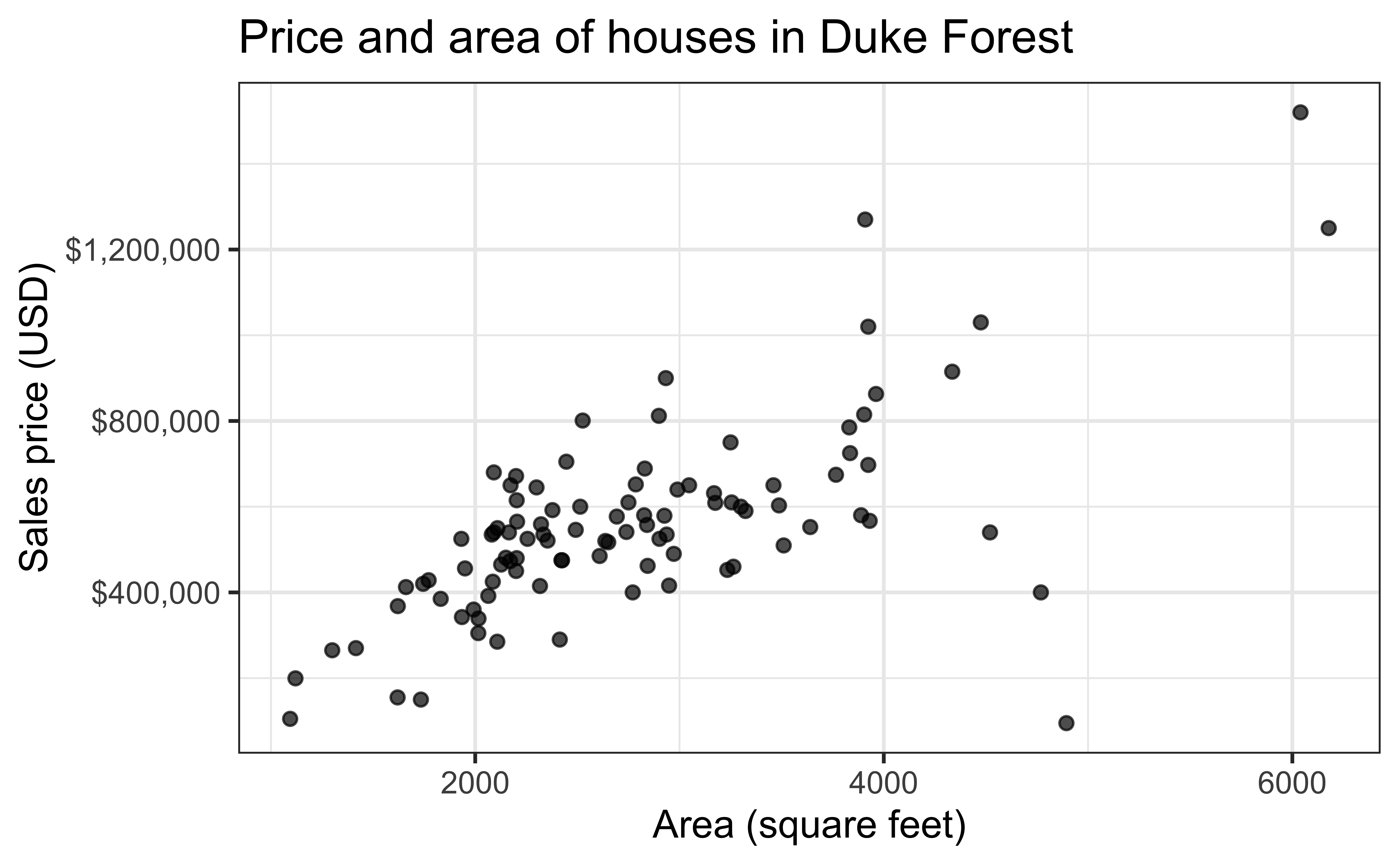

Modeling

df_fit <- lm(price ~ area, data = duke_forest)

tidy(df_fit) |>
  kable(digits = 2) #neatly format table to 2 digits

term	estimate	std.error	statistic	p.value
(Intercept)	116652.33	53302.46	2.19	0.03
area	159.48	18.17	8.78	0.00

. . .

Intercept: Duke Forest houses that are 0 square feet are expected to sell, for $116,652, on average.
- Is this interpretation meaningful?
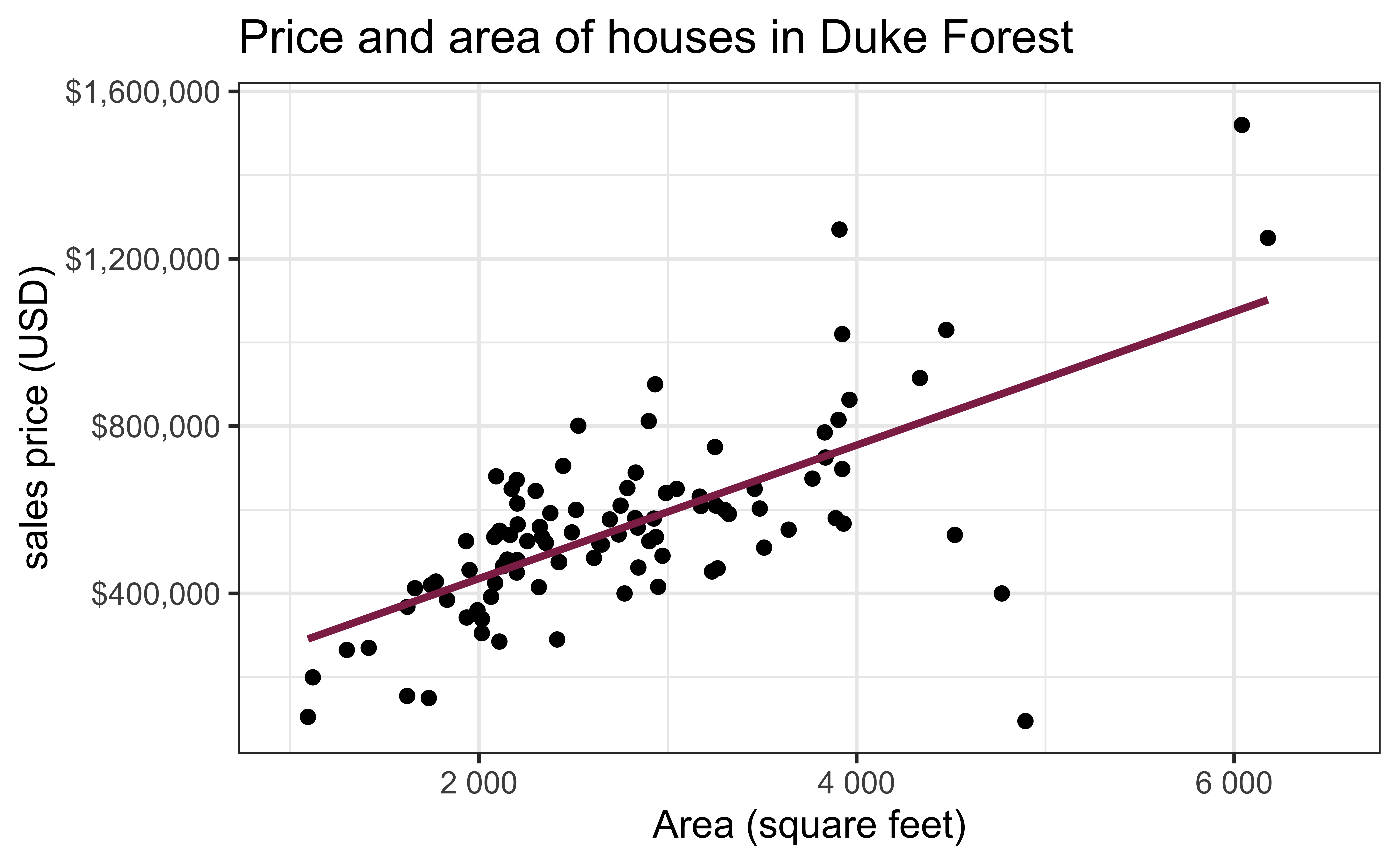
Slope: For each additional square foot, we expect the sales price of Duke Forest houses to be higher by $159, on average.

From sample to population

For each additional square foot, we expect the sales price of Duke Forest houses to be higher by $159, on average.

This estimate is valid for the single sample of 98 houses.
But what if we’re not interested quantifying the relationship between the size and price of a house in this single sample?
What if we want to say something about the relationship between these variables for all houses in Duke Forest?

Statistical inference

Statistical inference provides methods and tools so we can use the single observed sample to make valid statements (inferences) about the population it comes from
For our inferences to be valid, the sample should be representative (ideally random) of the population we’re interested in

Image source: Eugene Morgan © Penn State

Inference for simple linear regression

Compute a confidence interval for the slope, $\beta_1$
Conduct a hypothesis test for the slope, $\beta_1$

Note

We can use the same methods for inference on the intercept, $\beta_0$, but we are often not interested in inference on the intercept in practice.

Confidence interval for the slope

Confidence interval

A plausible range of values for a population parameter is called a confidence interval
Using only a single point estimate is like fishing in a murky lake with a spear, and using a confidence interval is like fishing with a net
- We can throw a spear where we saw a fish but we will probably miss, if we toss a net in that area, we have a good chance of catching the fish
- Similarly, if we report a point estimate, we probably will not hit the exact population parameter, but if we report a range of plausible values we have a good shot at capturing the parameter

Confidence interval for the slope

A confidence interval will allow us to make a statement like “For each additional square foot, the model predicts the sales price of Duke Forest houses to be higher, on average, by $159, plus or minus X dollars.”

. . .

Should X be $10? $100? $1000?
If we were to take another sample of 98 would we expect the slope calculated based on that sample to be exactly $159? Off by $10? $100? $1000?
The answer depends on how variable (from one sample to another sample) the sample statistic (the slope) is
We need a way to quantify the variability of the sample statistic

Quantify the variability of the slope

for estimation

Two approaches:
1. Via simulation (what we’ll do today)
2. Via theoretical results and mathematical models (what we’ll do in an upcoming class)
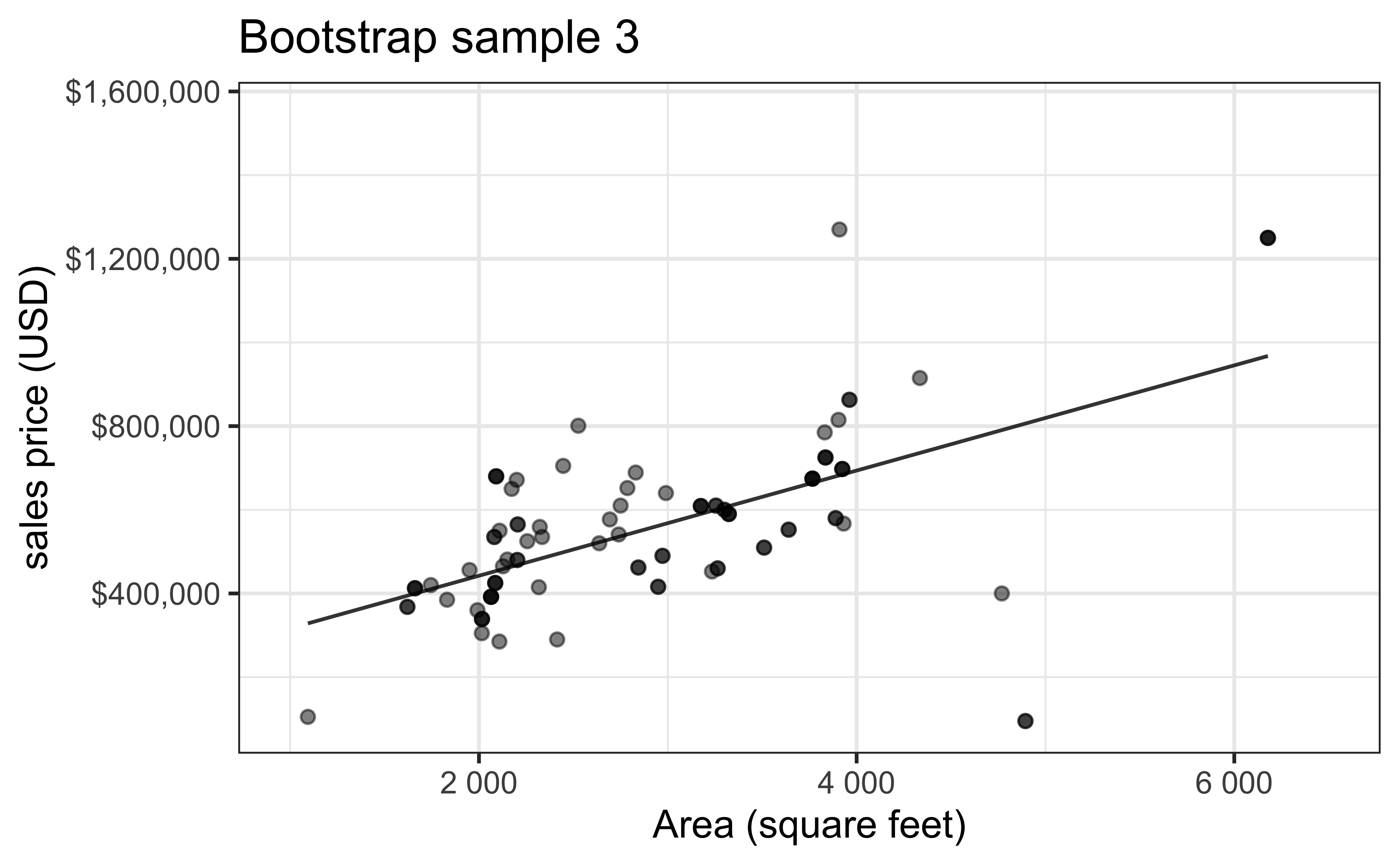
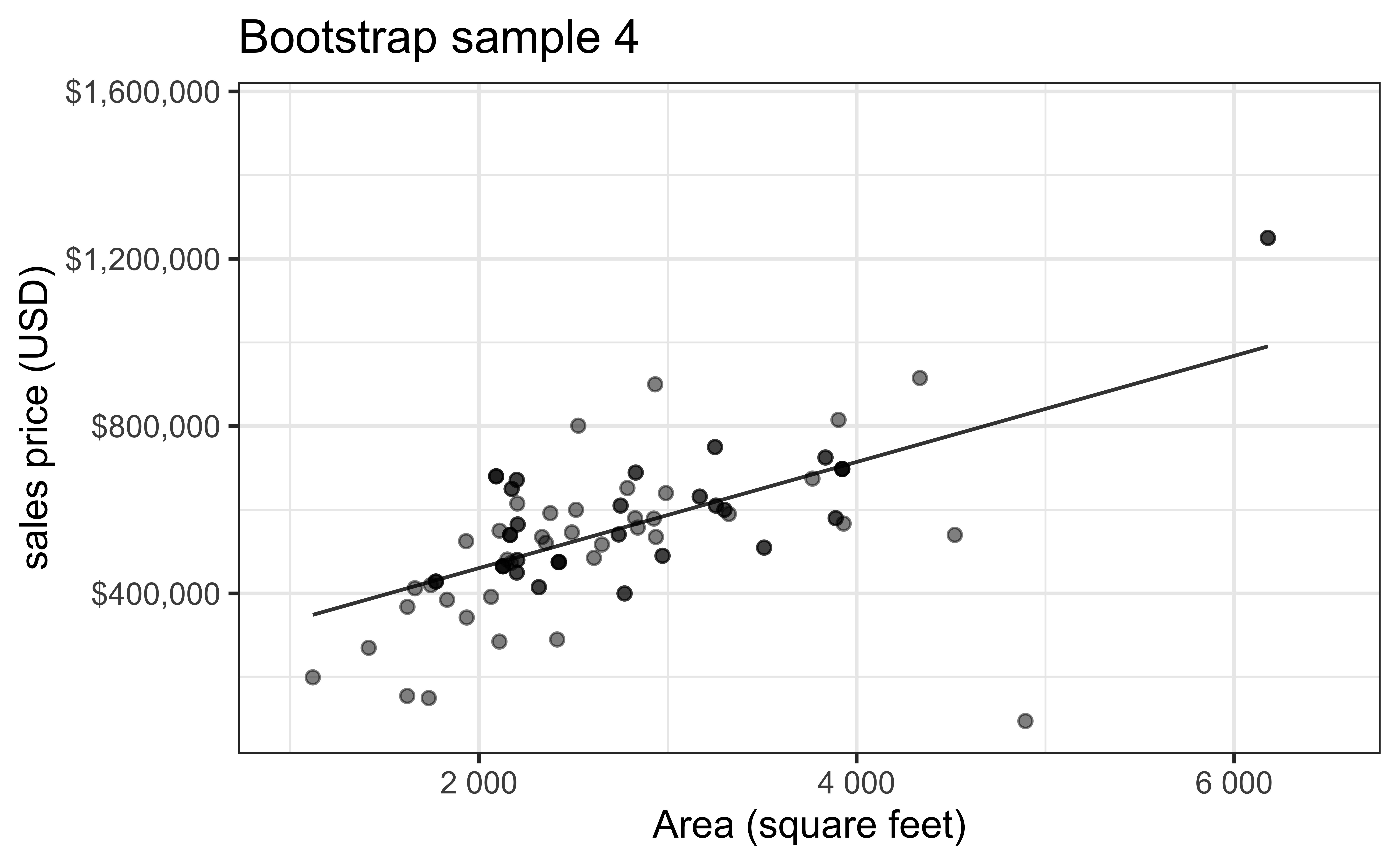
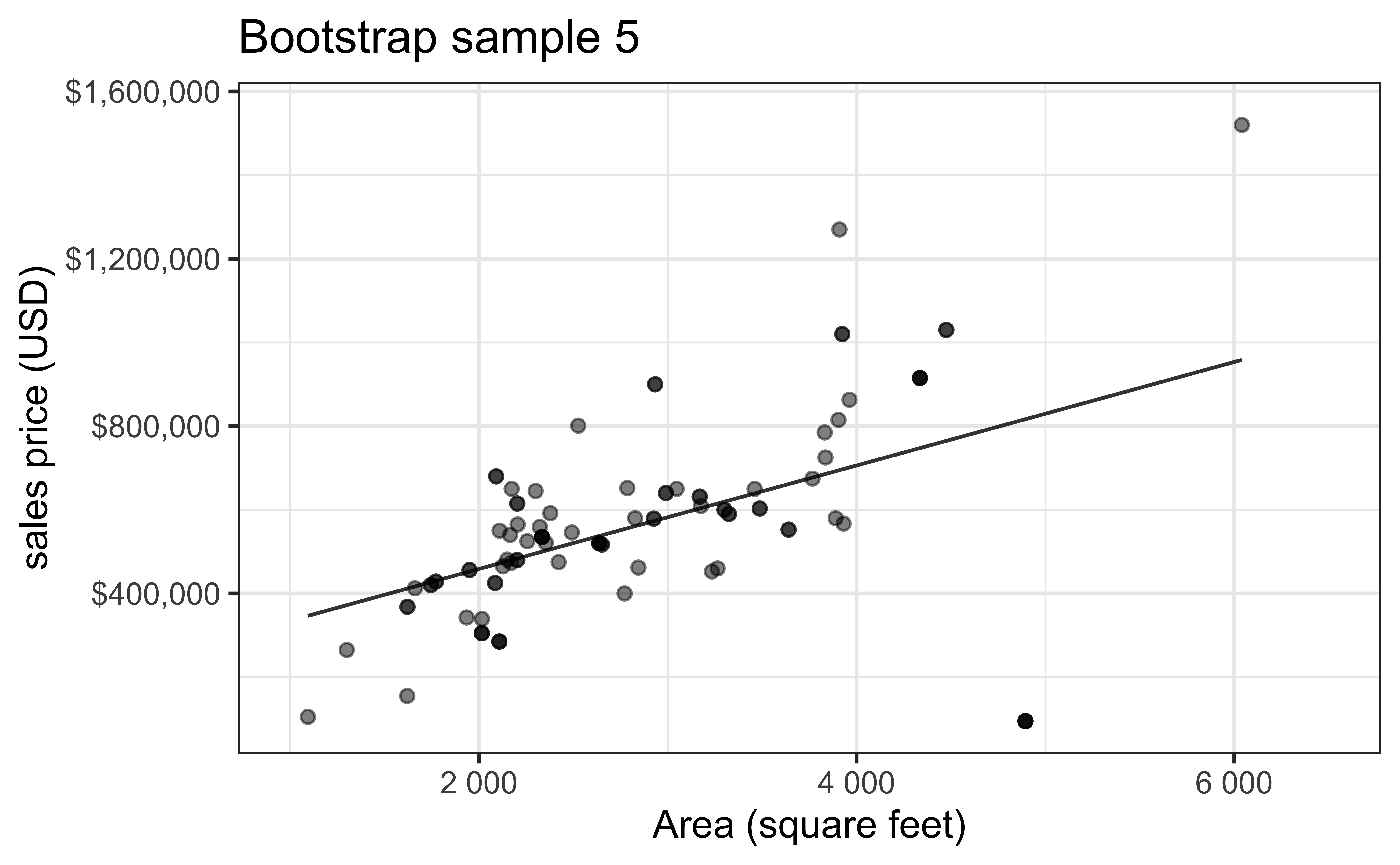
Bootstrapping to quantify the variability of the slope for the purpose of estimation:
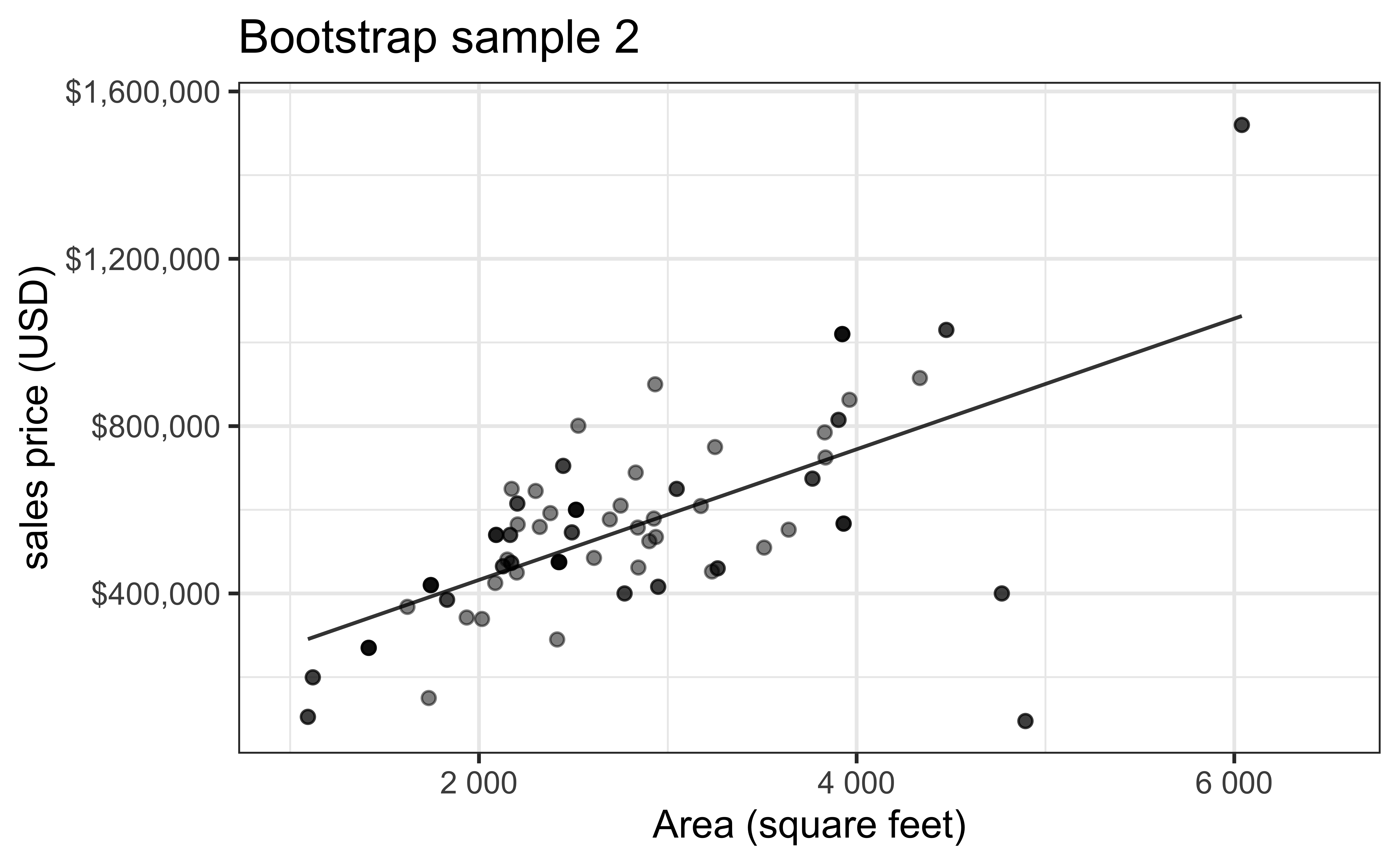
- Bootstrap new samples from the original sample, i.e. take sample of size $n$ with replacement
- Fit models to each of the samples and estimate the slope
- Use features of the distribution of the bootstrapped slopes to construct a confidence interval

Bootstrap sample 1

Bootstrap sample 2

Bootstrap sample 3

Bootstrap sample 4

Bootstrap sample 5

. . .

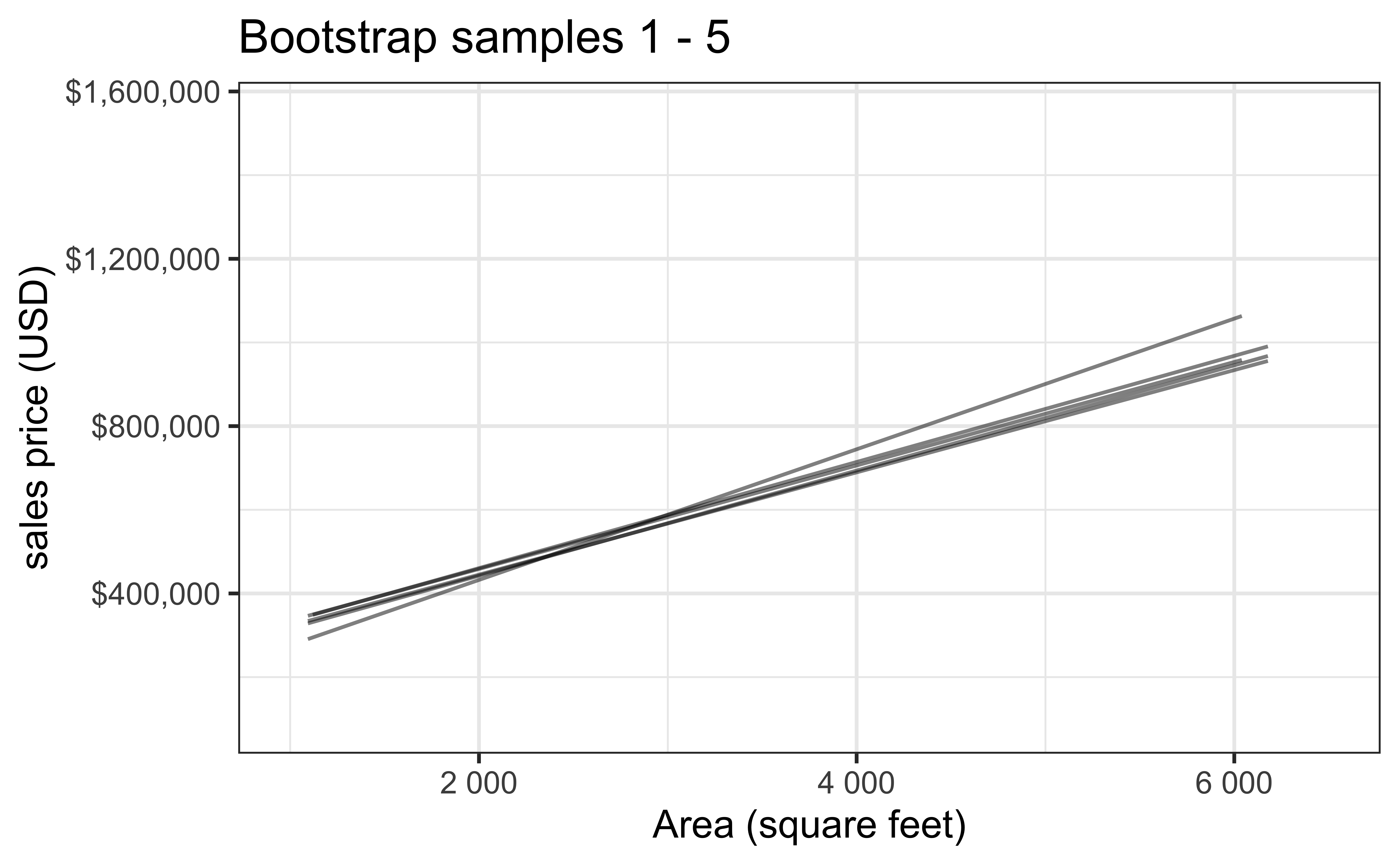
so on and so forth…

Bootstrap samples 1 - 5

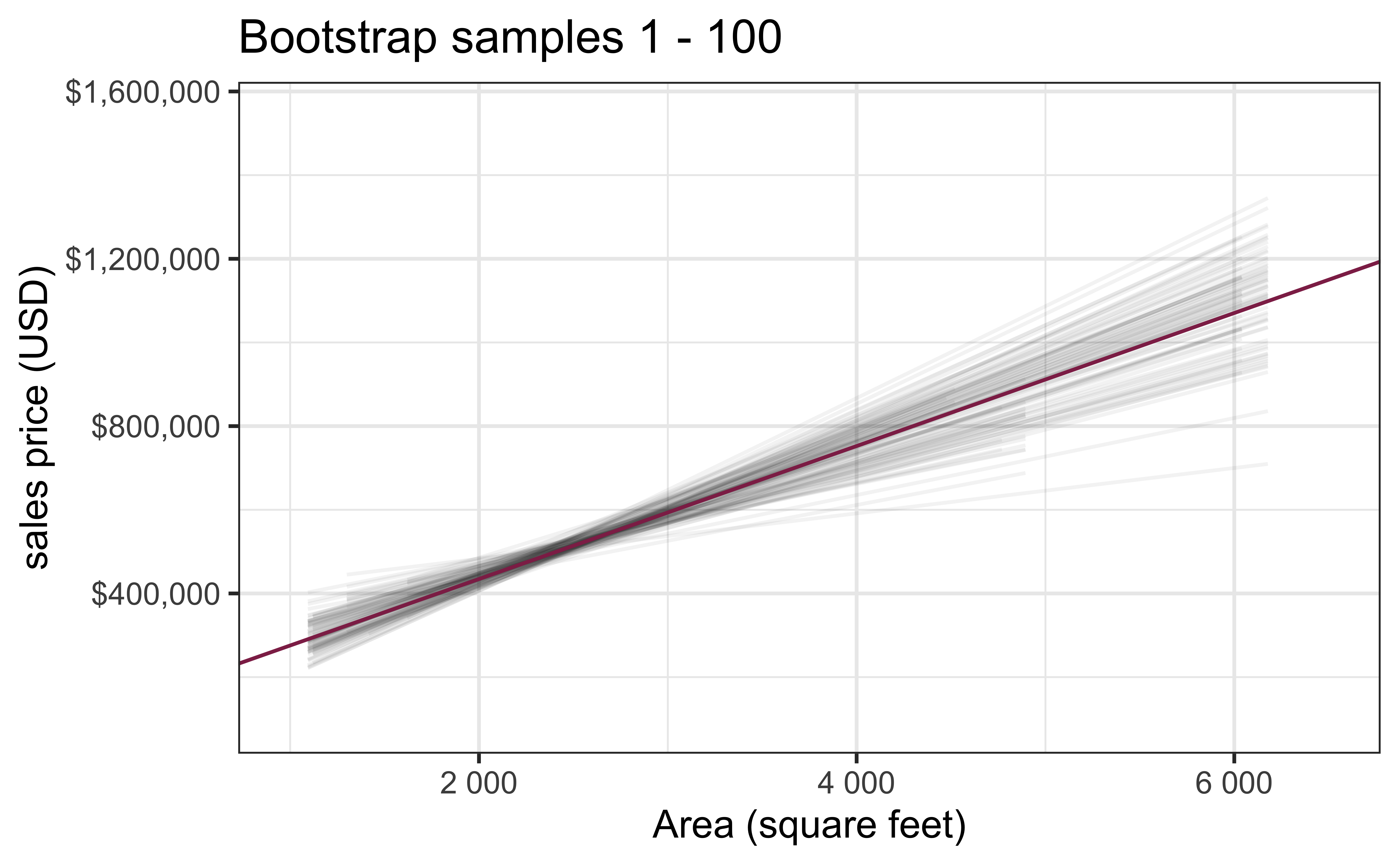
Bootstrap samples 1 - 100

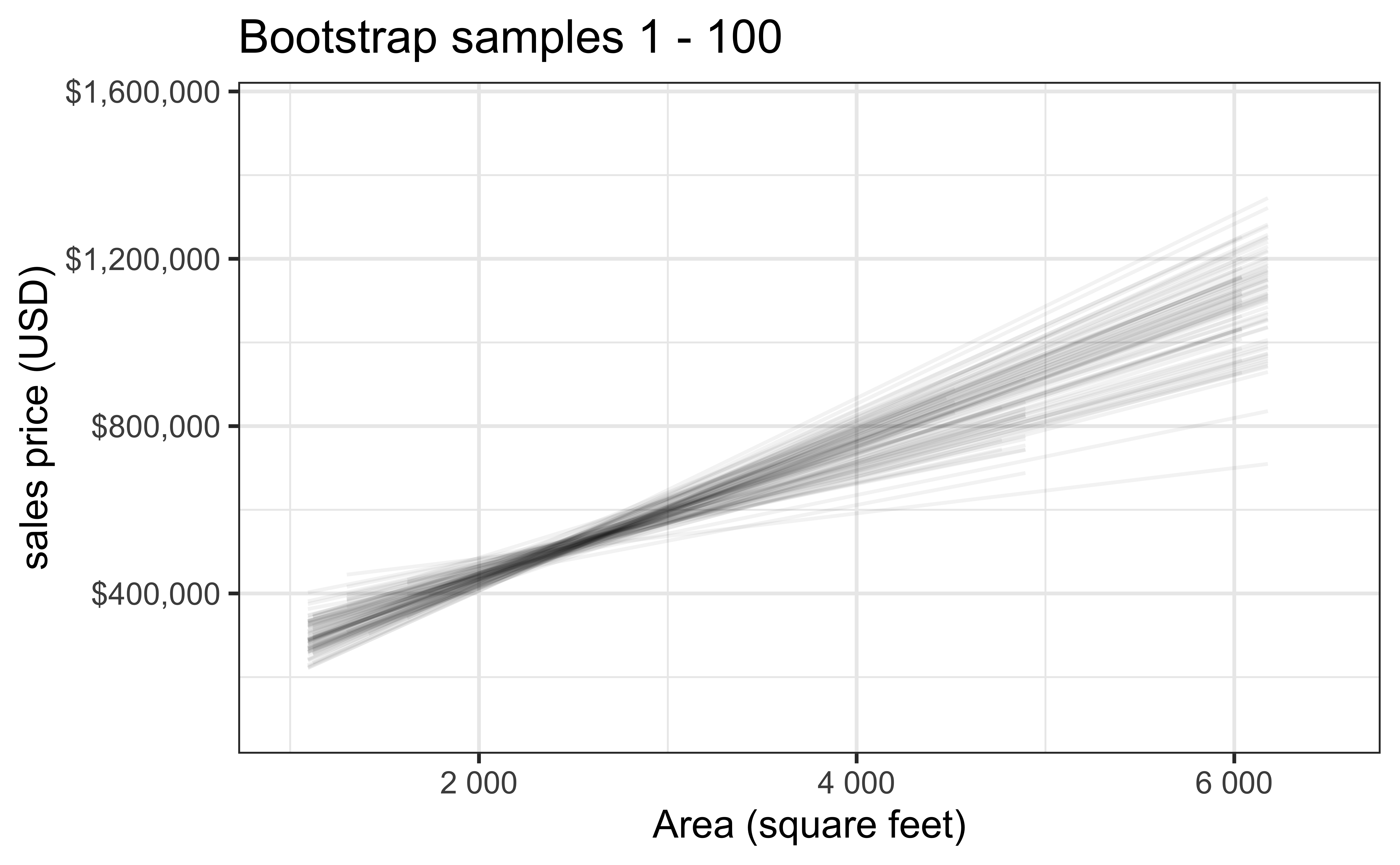
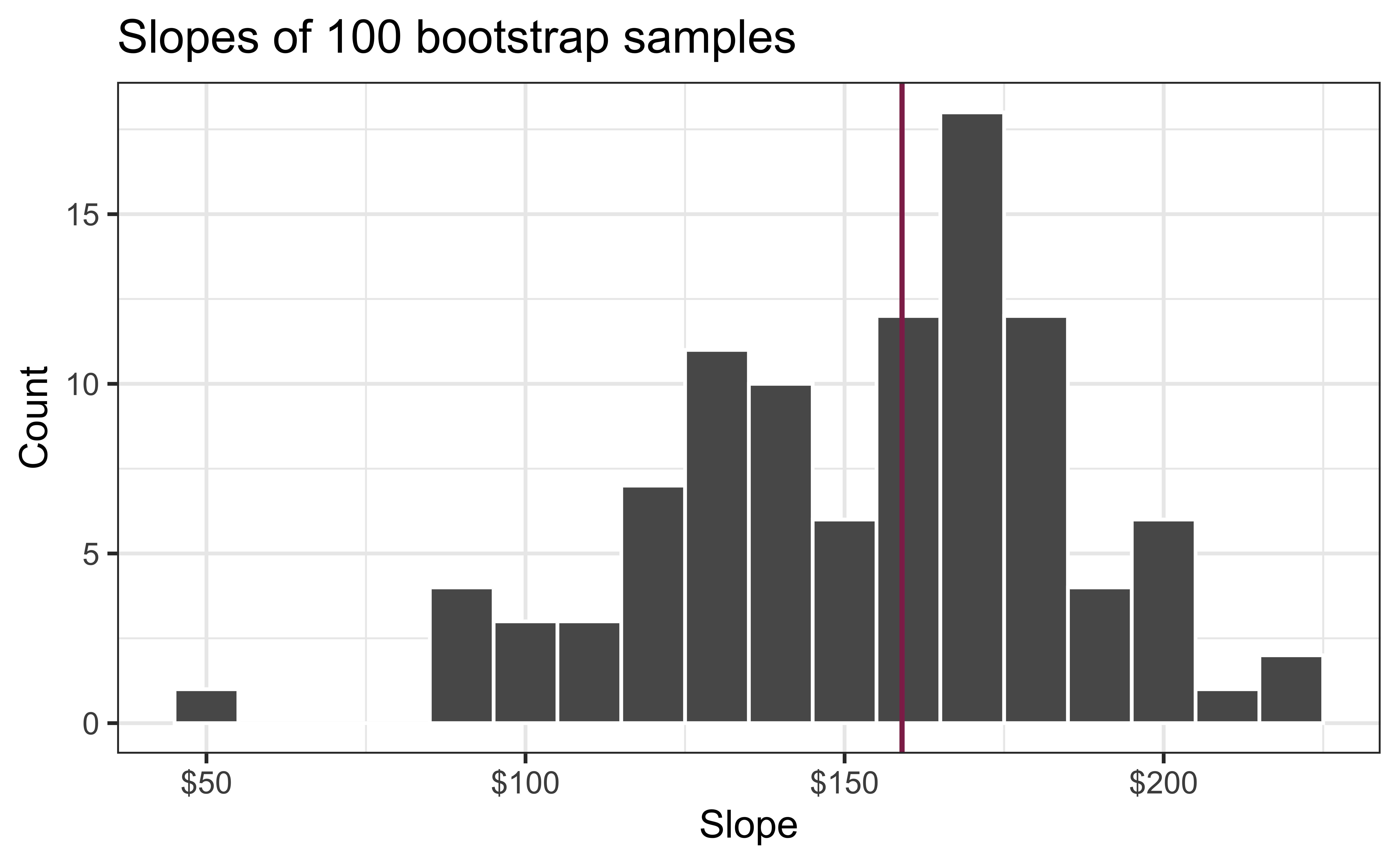
Slopes of bootstrap samples

Fill in the blank: For each additional square foot, the model predicts the sales price of Duke Forest houses to be higher, on average, by $159, plus or minus ___ dollars.

Slopes of bootstrap samples

Fill in the blank: For each additional square foot, we expect the sales price of Duke Forest houses to be higher, on average, by $159, plus or minus ___ dollars.

Bootstrap sampling distribution

Let’s increase the number of bootstrap samples to 1000. The bootstrap sampling distribution is the distribution of estimated slopes given samples of size $n$ (the same as our data).

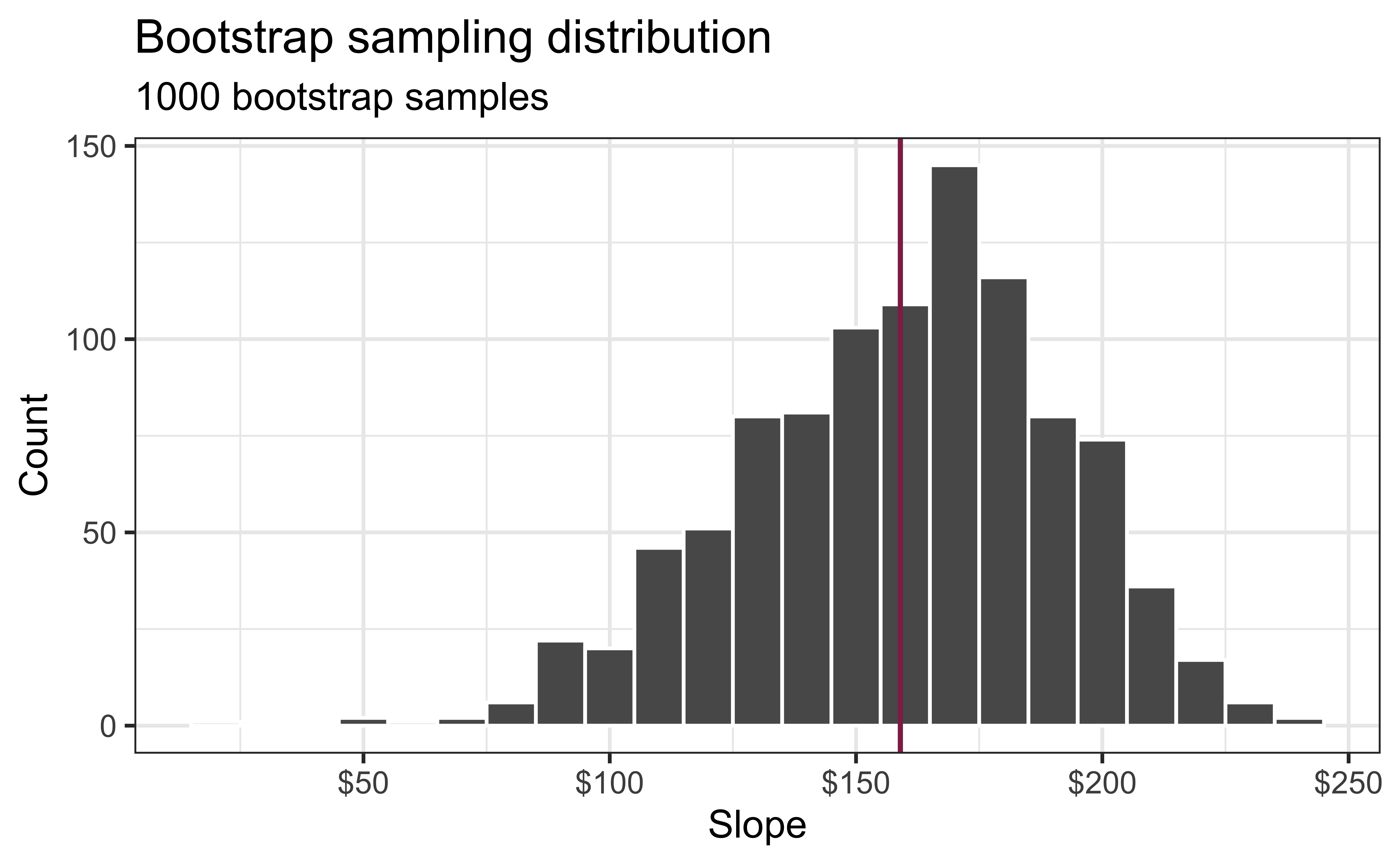
Bootstrap sampling distribution

What is the approximate center of the bootstrap sampling distribution?
The standard deviation of the bootstrap sampling distribution is 32.319. What does this value represent?

🔗 https://forms.office.com/r/naWVT11vBu

Confidence level

How confident are you that the true slope is between $0 and $250? How about $150 and $170? How about $90 and $210?

95% confidence interval

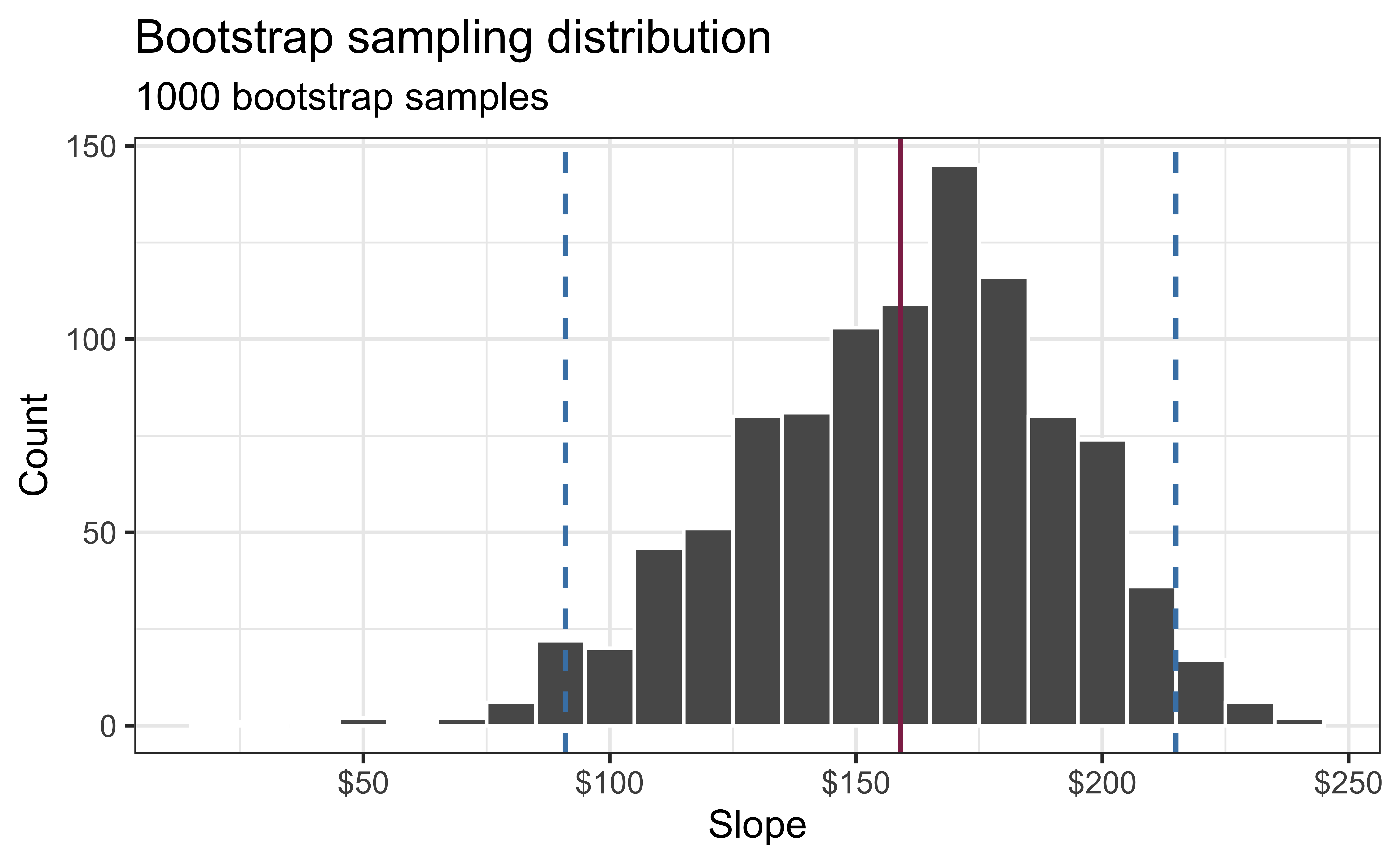
A 95% confidence interval is bounded by the middle 95% of the bootstrap distribution
We are 95% confident that for each additional square foot, sales price of Duke Forest houses to be higher, on average, by $90.97 to $214.93.

Computing the CI for the slope I

Calculate the observed slope:

observed_fit <- duke_forest |>
  specify(price ~ area) |>
  fit()

observed_fit

# A tibble: 2 × 2
  term      estimate
  <chr>        <dbl>
1 intercept  116652.
2 area          159.

Computing the CI for the slope II

Take 100 bootstrap samples and fit models to each one:

set.seed(1120)

boot_fits <- duke_forest |>
  specify(price ~ area) |>
  generate(reps = 100, type = "bootstrap") |>
  fit()

boot_fits

# A tibble: 200 × 3
# Groups:   replicate [100]
   replicate term      estimate
       <int> <chr>        <dbl>
 1         1 intercept   47819.
 2         1 area          191.
 3         2 intercept  144645.
 4         2 area          134.
 5         3 intercept  114008.
 6         3 area          161.
 7         4 intercept  100639.
 8         4 area          166.
 9         5 intercept  215264.
10         5 area          125.
# ℹ 190 more rows

Use ~ 100 bootstrap samples to write code, and 1000+ samples for final analysis results.

Computing the CI for the slope III

Percentile method: Compute the 95% CI as the middle 95% of the bootstrap distribution:

get_confidence_interval(
  boot_fits, 
  point_estimate = observed_fit, 
  level = 0.95,
  type = "percentile" #default method
)

# A tibble: 2 × 3
  term      lower_ci upper_ci
  <chr>        <dbl>    <dbl>
1 area          92.1     223.
2 intercept -36765.   296528.

Precision vs. accuracy

If we want to be very certain that we capture the population parameter, should we use a wider or a narrower interval? What drawbacks are associated with using a wider interval?

. . .

Precision vs. accuracy

How can we get best of both worlds – high precision and high accuracy?

. . .

Consider a 90%, 95%, and 99% confidence interval.

Which interval is most precise?
Which is most accurate?

Changing confidence level

## confidence level: 90%
get_confidence_interval(
  boot_fits, point_estimate = observed_fit, 
  level = 0.90, type = "percentile"
)

# A tibble: 2 × 3
  term      lower_ci upper_ci
  <chr>        <dbl>    <dbl>
1 area          104.     212.
2 intercept  -24380.  256730.

## confidence level: 99%
get_confidence_interval(
  boot_fits, point_estimate = observed_fit, 
  level = 0.99, type = "percentile"
)

# A tibble: 2 × 3
  term      lower_ci upper_ci
  <chr>        <dbl>    <dbl>
1 area          56.3     226.
2 intercept -61950.   370395.

Recap

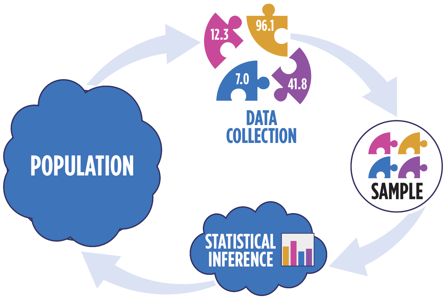
Population: Complete set of observations of whatever we are studying, e.g., people, tweets, photographs, etc. (population size = $N$)
Sample: Subset of the population, ideally random and representative (sample size = $n$)
Sample statistic $\ne$ population parameter, but if the sample is good, it can be a good estimate
Statistical inference: Discipline that concerns itself with the development of procedures, methods, and theorems that allow us to extract meaning and information from data that has been generated by stochastic (random) process
We report the estimate with a confidence interval, and the width of this interval depends on the variability of sample statistics from different samples from the population
Since we can’t continue sampling from the population, we bootstrap from the one sample we have to estimate sampling variability

For next class

Simulation-based inference: Permutation tests
Complete Lecture 05 prepare