library(tidyverse)
library(tidymodels)
library(knitr)
library(patchwork)

rail_trail <- read_csv("data/rail-trail.csv")AE 07: Exam 01 review
Trail users
Important
Go to the course GitHub organization and locate your ae-07 repo to get started.
One person from each group: Put your group’s response on your slide: https://docs.google.com/presentation/d/15nF9ADDlQwiDiRG55TCMOkqQgCy6_JB5hjPKE_kZE90/edit?usp=sharing
Packages
Trail users
The Pioneer Valley Planning Commission (PVPC) collected data for ninety days from April 5, 2005 to November 15, 2005. Data collectors set up a laser sensor, with breaks in the laser beam recording when a rail-trail user passed the data collection station.
We will use regression analysis to predict the number of trail users based on weather and other features describing the day.
We’ll use the following variables in this analysis:
volumeestimated number of trail users that day (number of breaks recorded)hightempdaily high temperature (in degrees Fahrenheit)daytypeone of “weekday” or “weekend”
View the data set1 to see the remaining variables.
Bivariate EDA
p1 <- ggplot(data = rail_trail, aes(x = hightemp, y = volume)) +
  geom_point() +
  labs(x = "High temperature (in Fahrenheit)",
       y = "Number of users",
       title = "Volume versus high temperature")

p2 <- ggplot(data = rail_trail, aes(x = daytype, y = volume)) +
  geom_boxplot() +
  labs(x = "",
       y = "Number of users",
       title = "Volume versus day type")

p1 + p2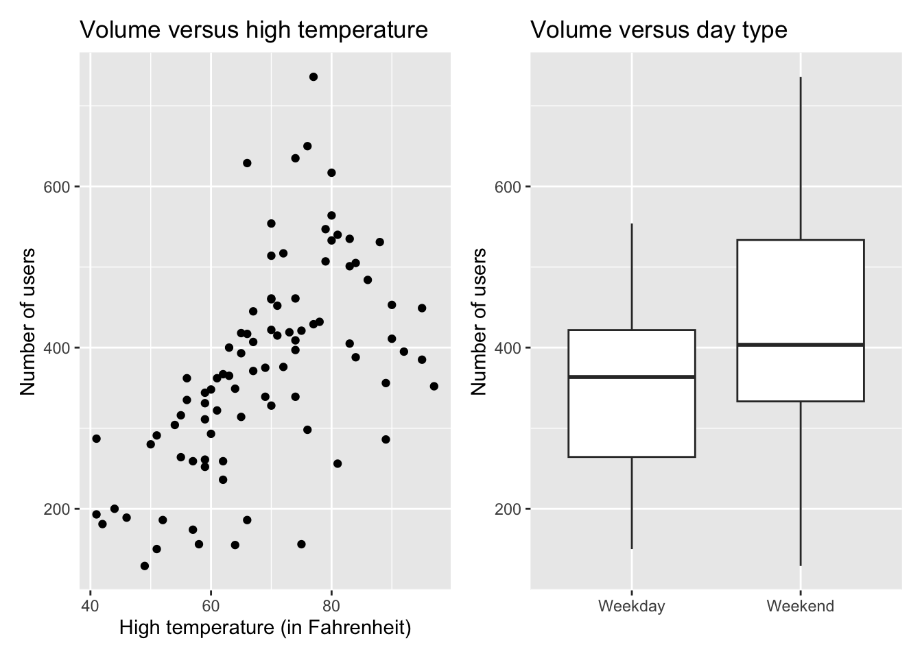
Models
Below is the code for the two models used in this analysis.
# main effects model
main_effects_model <- lm(volume ~ hightemp + daytype, data = rail_trail)


# interaction model
interaction_model <- lm(volume ~ hightemp + daytype + hightemp * daytype,
                         data = rail_trail)
Exercises
Exercise 1
Consider the main effects model.
- Display the model along with the 90% confidence intervals for the coefficients.
Interpret the coefficient of
hightempin the context of the data.Interpret the coefficient of
daytypeWeekendin the context of the data.Does the intercept have a meaningful interpretation? Explain your reasoning.
If not, what can we do to make the interpretation meaningful?
Exercise 2
Consider the interactions effects model.
- Display the model along with the 90% confidence intervals for the coefficients.
Interpret the main effect of
hightemp.Interpret the coefficient
hightemp:daytypeWeekend.According to this model, does the effect of
hightempdiffer for weekends vs. weekdays? Explain.
Exercise 3
The following code can be used to create a bootstrap distribution for the model coefficients in the main effects model.
- Describe what each line of code does.
- 1
- ___
- 2
- ___
- 3
- ___
- 4
- ___
How many observations are in each bootstrap sample?
Explain why we use bootstrap sampling, instead of permutation sampling, to construct confidence intervals.
Exercise 4
Consider the bootstrap distribution for the coefficient of hightemp in the main effects model.
How many estimated coefficients of
hightempmake up the bootstrap distribution?Run the code from the previous exercise to construct the bootstrap distribution. Use the bootstrap distribution to compute \(SE_{\hat{\beta}_\text{hightemp}}\). Explain what this value means in the context of the data.
Construct a 90% bootstrap confidence interval for the coefficient of
hightemp. Interpret the interval in the context of the data.
Exercise 5
We would like to conduct the following hypothesis test for the main effects model.
\[ \begin{aligned} &H_0: \beta_\text{hightemp} = 0 \\ &H_a: \beta_\text{hightemp} \neq 0 \end{aligned} \]
State the hypotheses in words.
Conduct a permutation test by permuting the response variable. Use 100 iterations, a seed of 210, and a significance level of \(\alpha = 0.05\).
Exercise 6
Use the interaction effects model to predict the volume for a Saturday that has a high temperature of 75 degrees Fahrenheit.
Suppose you’re asked to construct a confidence interval and a prediction interval given a Saturday with a high temperature of 75 degrees Fahrenheit. Which interval would you expect to be wider and why? In your answer clearly state the difference between these intervals.
Construct the 90% intervals and interpret them in the context of the data.
Wrapping up
Important
Once you’ve completed the AE:
Render the document to produce the PDF with all of your work from today’s class.
Push all your work to your AE repo on GitHub. You’re done! 🎉
Footnotes
Source: Pioneer Valley Planning Commission via the mosaicData package.↩︎