Model conditions + diagnostics
Feb 10, 2026
Permutation illustrated
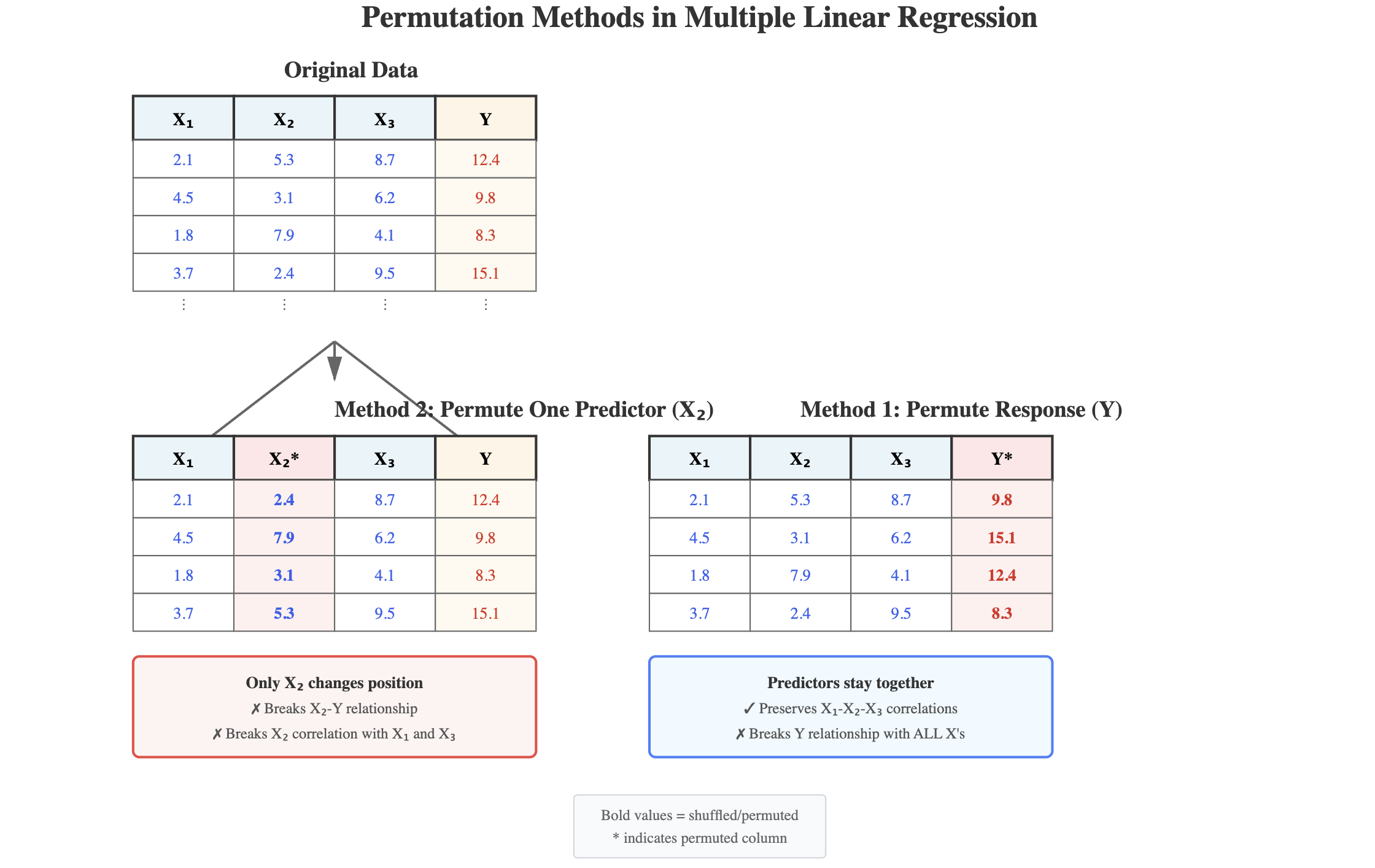
Generate from Claude AI Sonnet 4.5 using the prompt: “Please draw a picture illustrating permuting the response variable versus permuting individual predictor variables.”
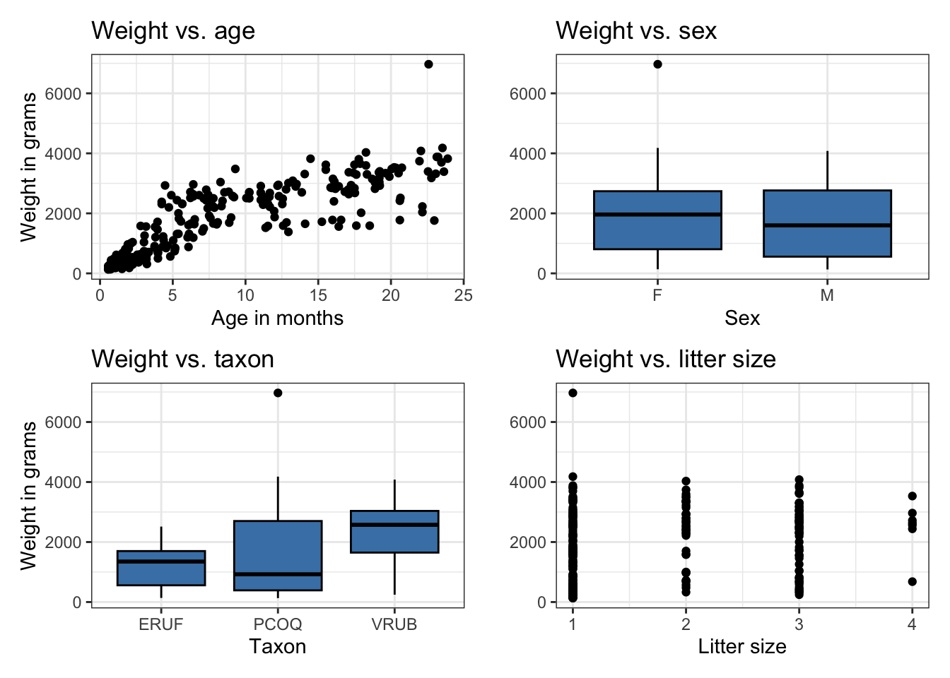
Bivariate EDA
Linearity
- Look at plot of residuals versus fitted (predicted) values.
- Linearity is satisfied if there is no discernible pattern in the plot (i.e., points randomly scattered around \(\text{residuals} = 0\))

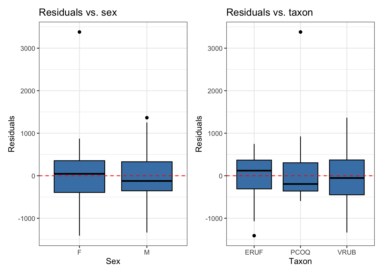
Residuals vs. predictors
If we need a closer look at the linearity condition, we can plot the residuals versus each quantitative predictor.
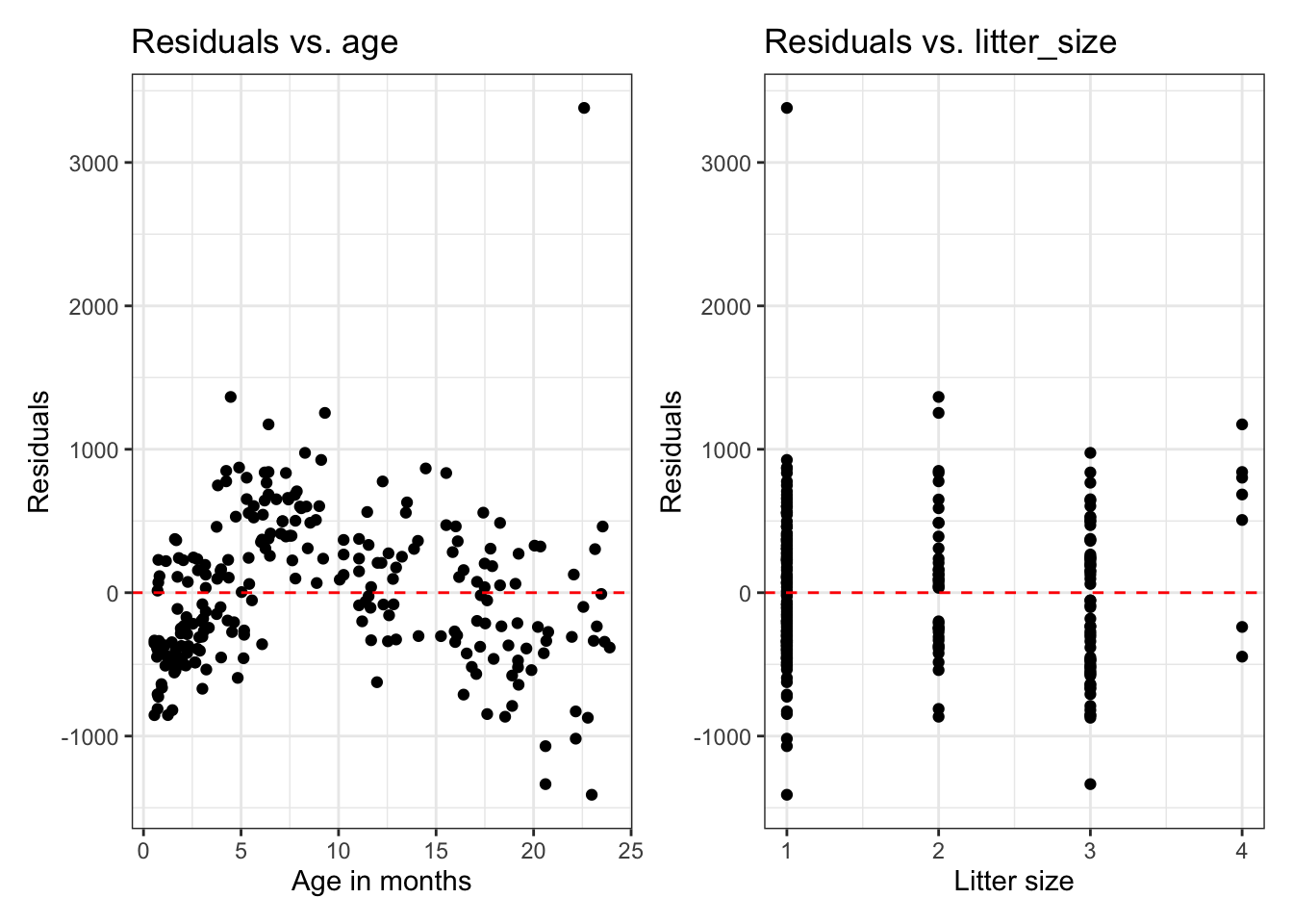
Example: Linearity not satisfied
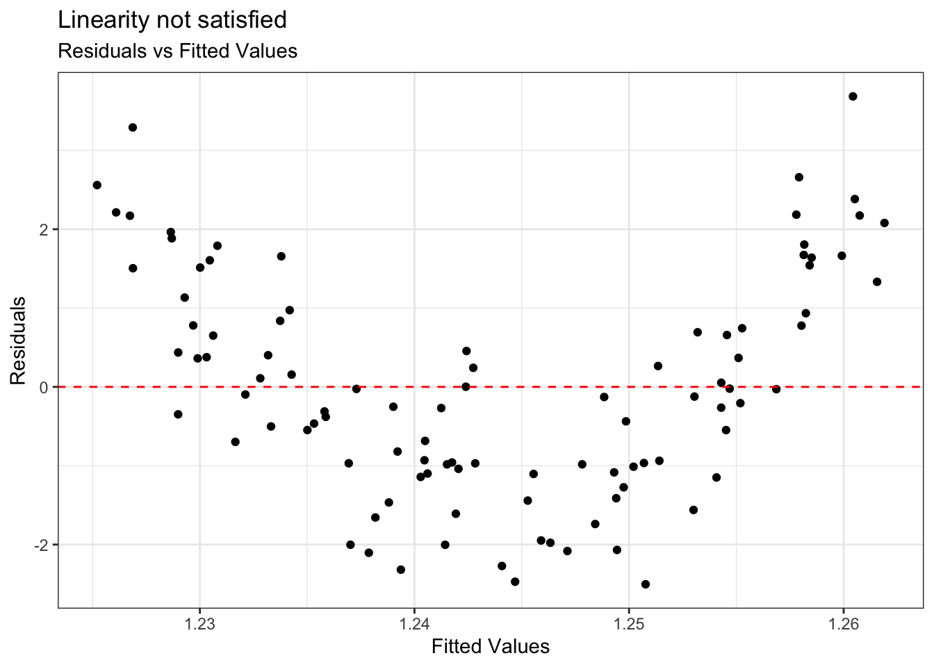
- If linearity is not satisfied, examine the plots of residuals versus each predictor.
- Add higher order term(s), as needed.
Equal variance
- Look at plot of residuals versus fitted (predicted) values.
- Equal variance is satisfied if the vertical spread of the points is approximately equal for all fitted values

Example: Equal variance not satisfied
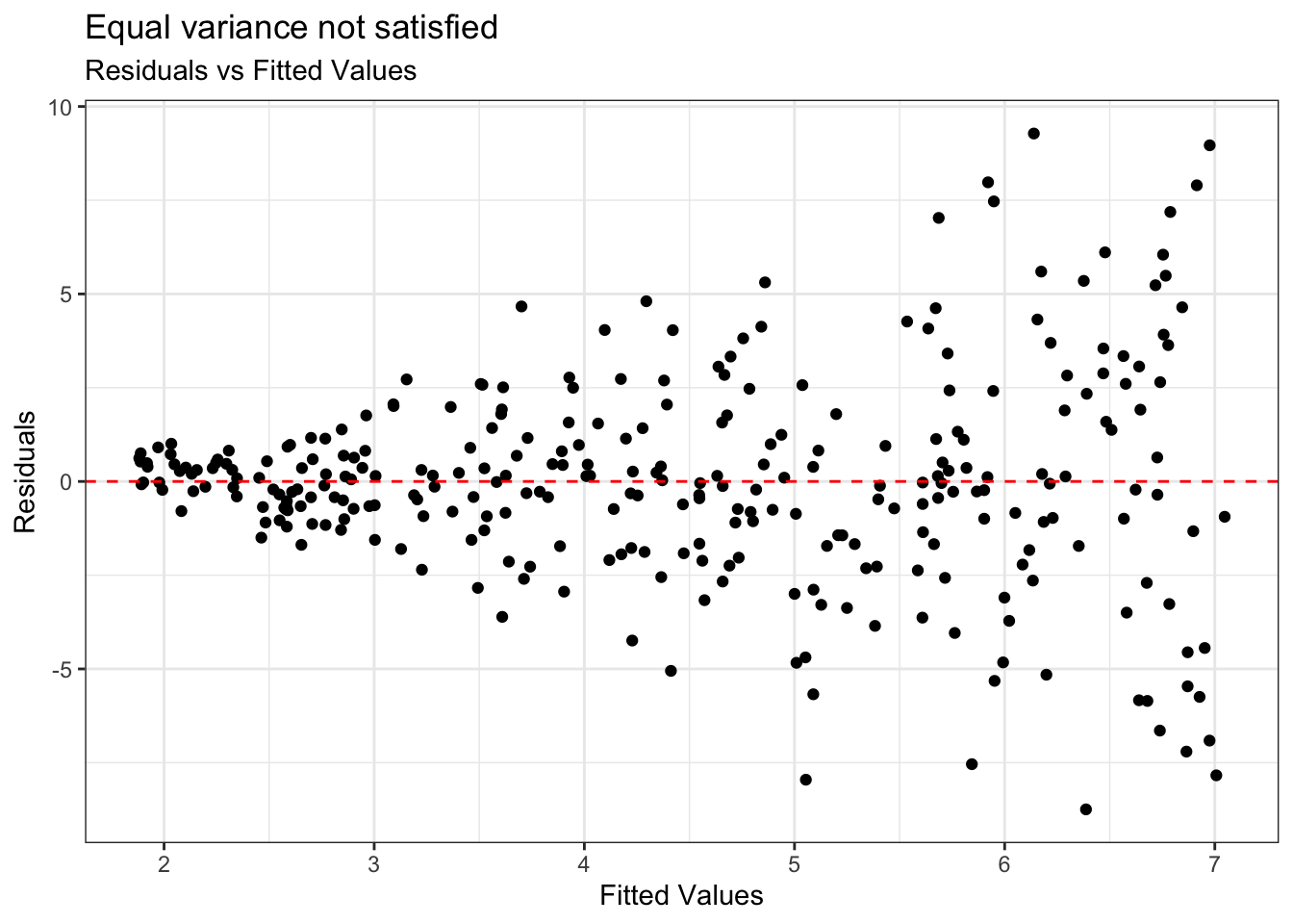
Condition is critical for inference
Address violations by applying transformation on the response
Normality
- Look at the distribution of the residuals
- Normality is satisfied if the distribution is approximately unimodal and symmetric. Inference robust to violations if \(n > 30\)
`stat_bin()` using `bins = 30`. Pick better value `binwidth`.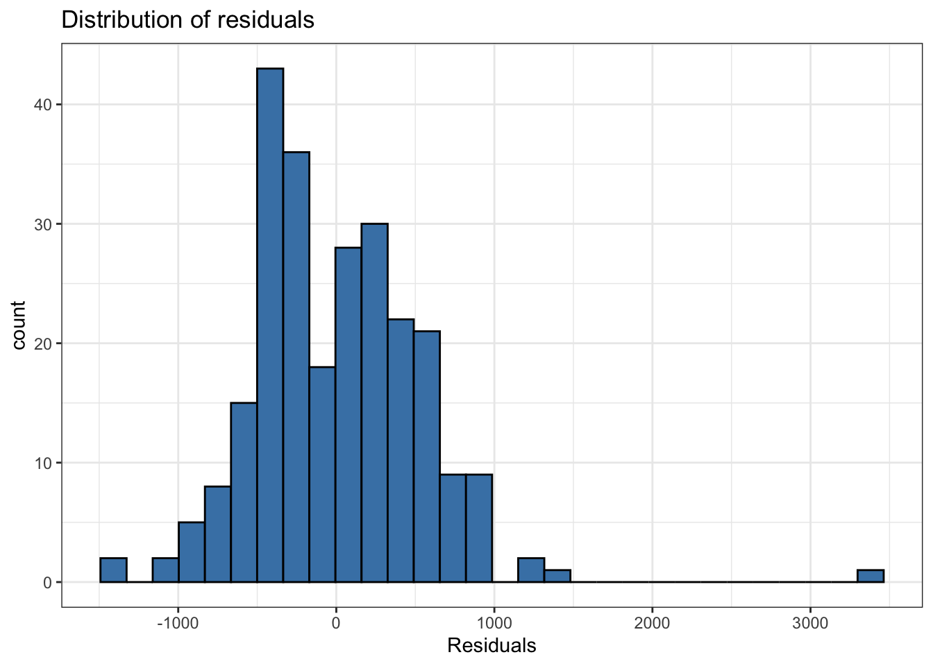
Independence
Influential Point
An observation is influential if removing has a noticeable impact on the regression coefficients
`geom_smooth()` using formula = 'y ~ x'
`geom_smooth()` using formula = 'y ~ x'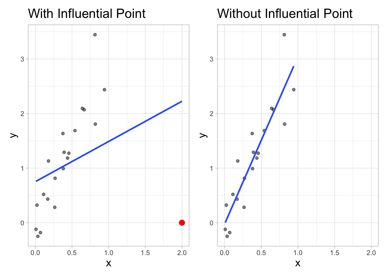
Let’s look at the data
`stat_bin()` using `bins = 30`. Pick better value `binwidth`.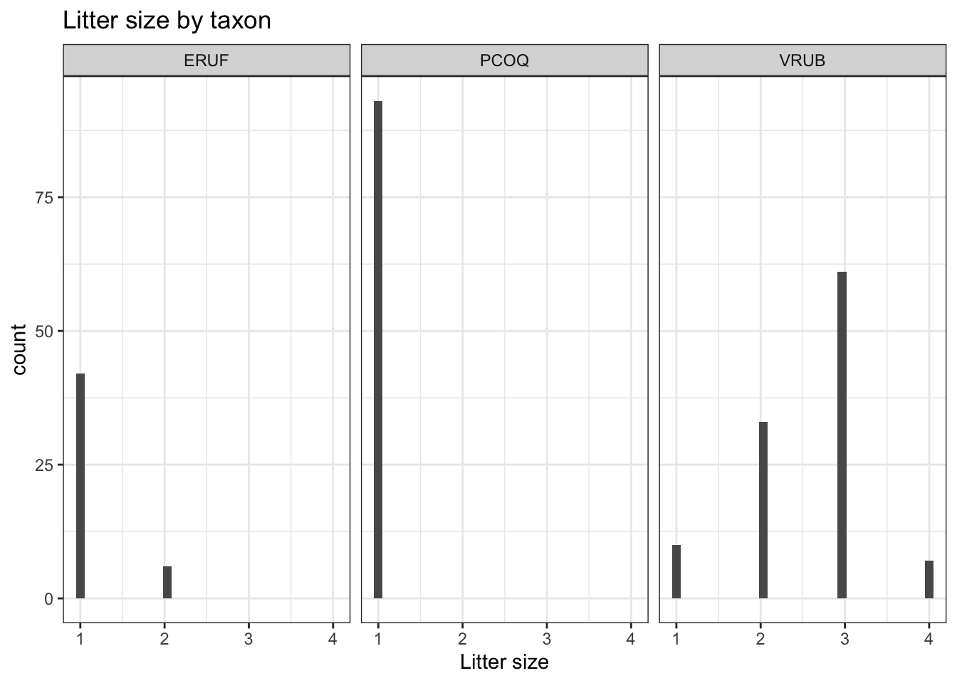
The high leverage points are primarily VRUB lemurs with no siblings.
Using standardized residuals
We can examine the standardized residuals directly from the output from the augment() function
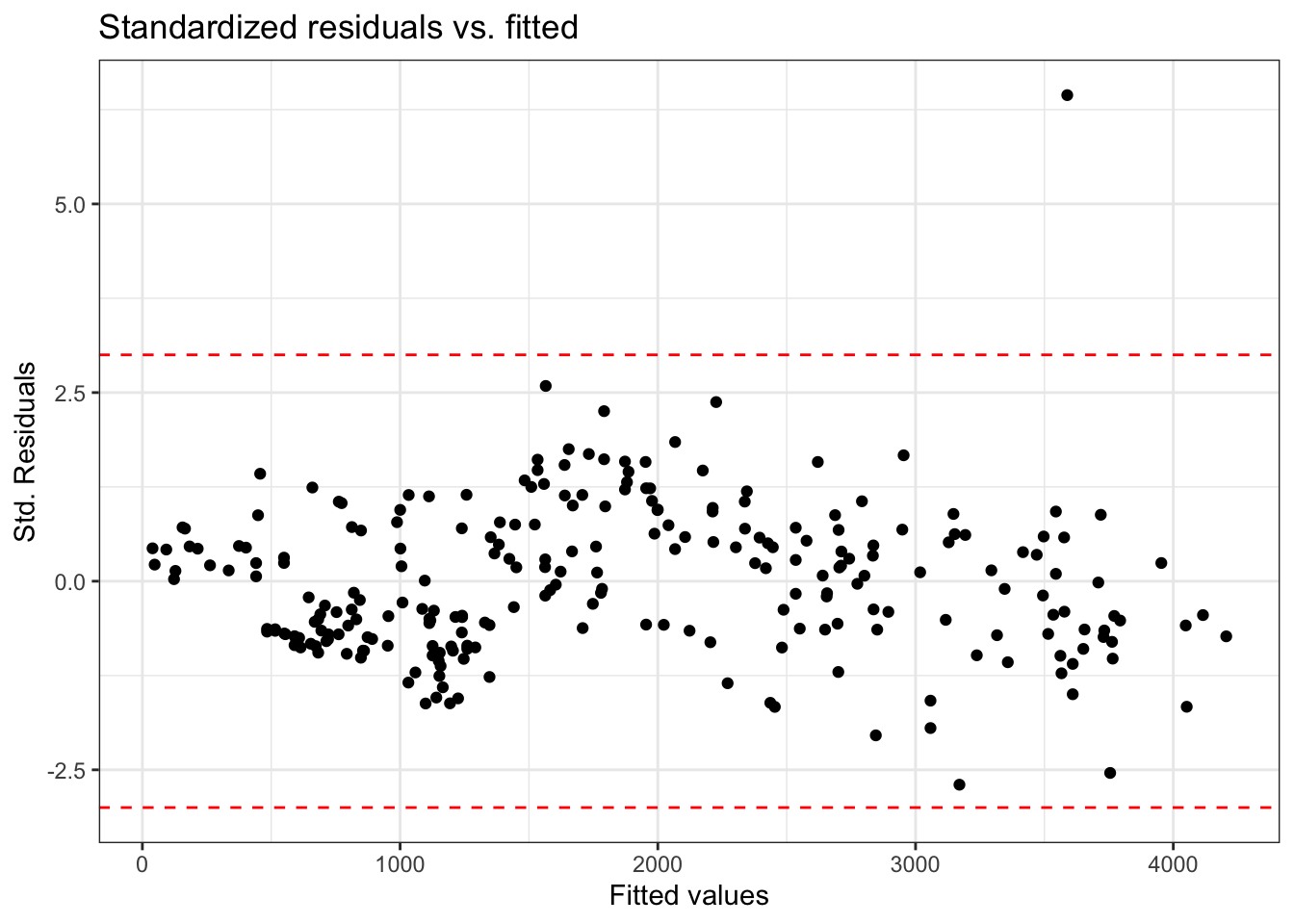
- An observation is a potential outlier if its standardized residual is beyond \(\pm 3\)
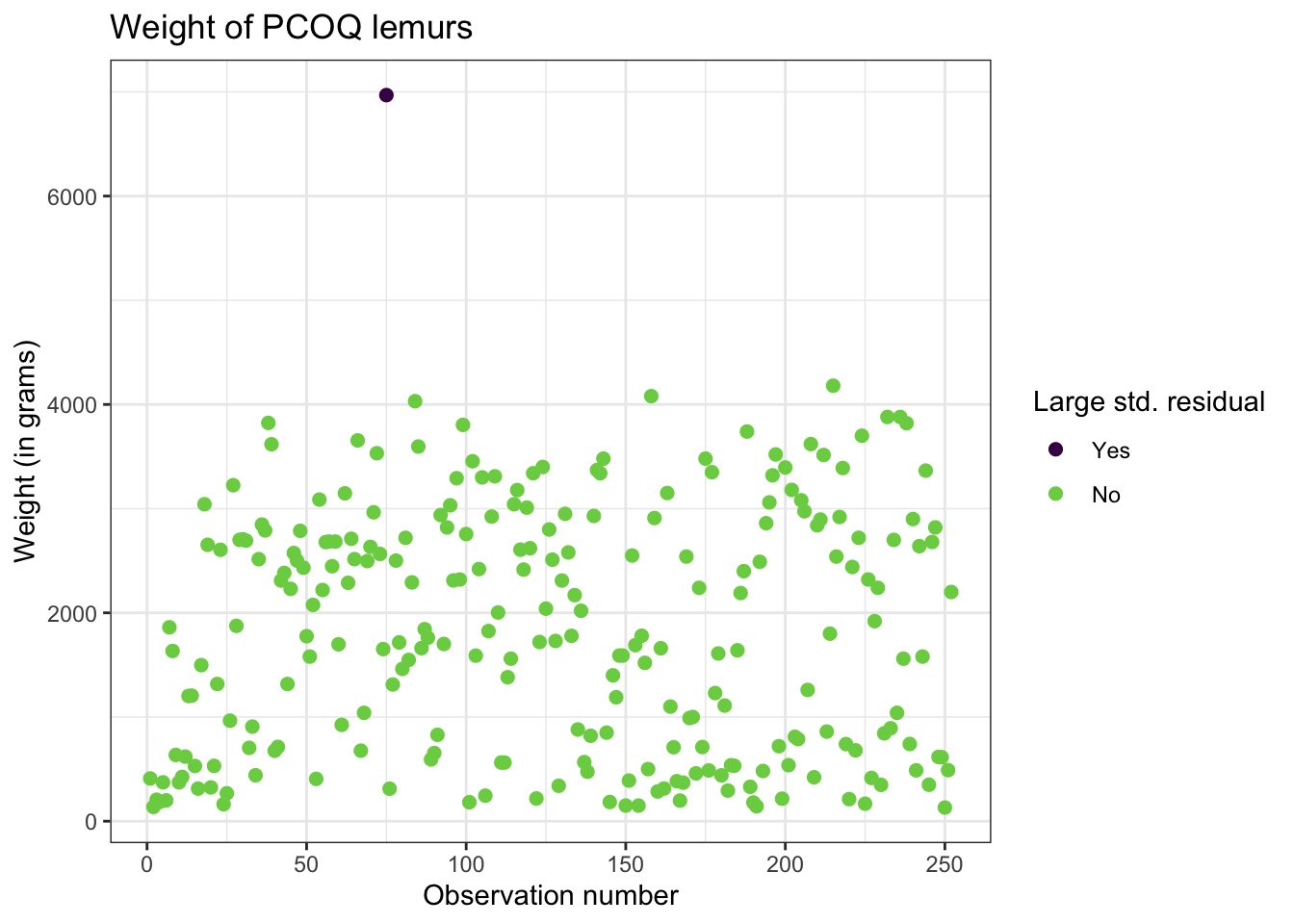
Digging in to the data
Let’s look at the value of the response variable to better understand potential outliers
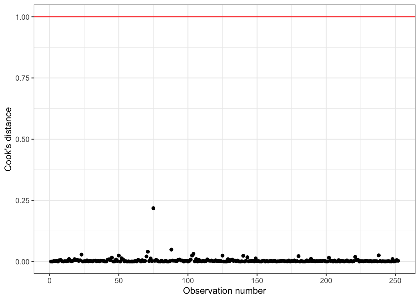
Cook’s Distance
Cook’s Distance is in the column .cooksd in the output from the augment() function