Lab 03
Multiple linear regression
Feb 09, 2026
Bivariate EDA
Code
p1 <- ggplot(data = football, aes(x = enrollment_th, y = total_exp_m)) +
  geom_point() +
  labs(x = "Enrollment (in thousands)",
       y = "Total expenditures (in millions)",
       title = "Football expenditures vs. enrollment")

p2 <- ggplot(data = football, aes(x = type, y = total_exp_m)) +
  geom_boxplot() +
  labs(x = "Institution type",
       y = "Total expenditures (in millions)",
       title = "Football expenditures vs. institution type")

p1 + p2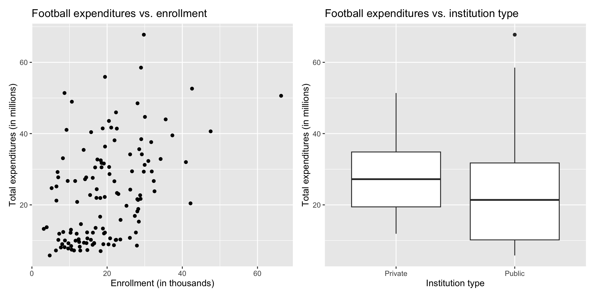
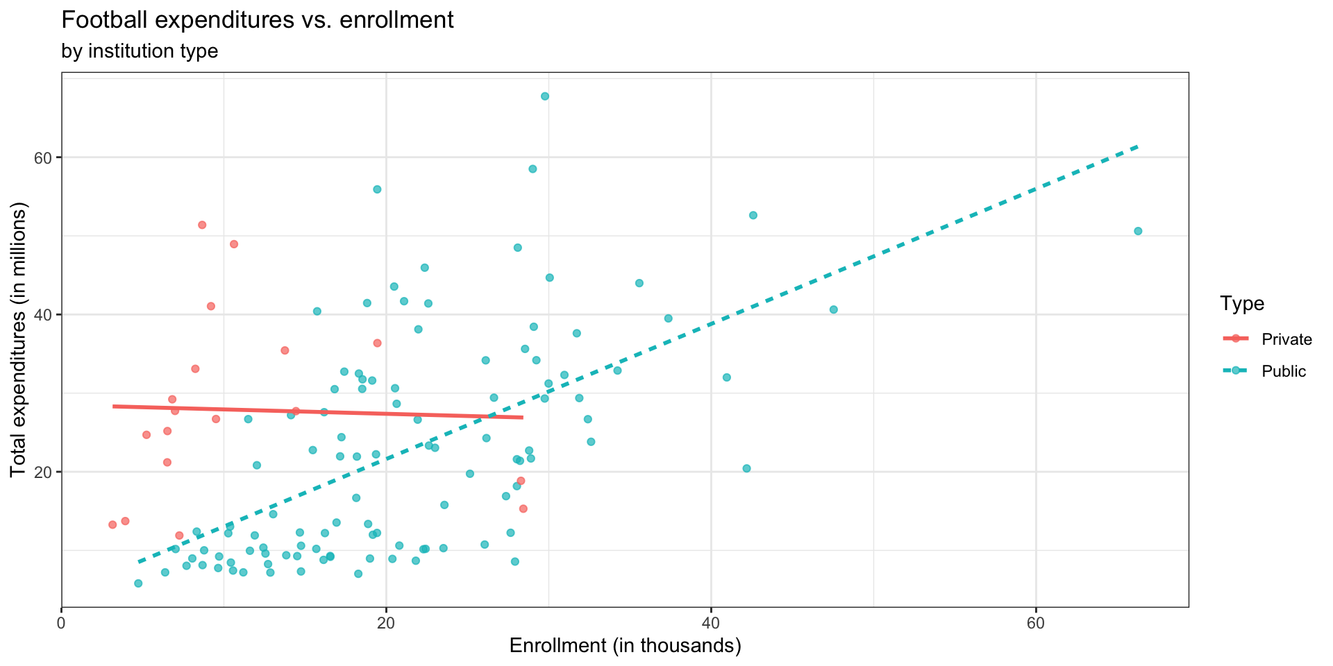
Potential interaction effect?
Code
ggplot(data = football, aes(x = enrollment_th, y = total_exp_m, color = type,
                            linetype = type)) +
  geom_point(alpha = 0.7) +
  geom_smooth(method = "lm", se = FALSE) +
  labs(x = "Enrollment (in thousands)",
       y = "Total expenditures (in millions)",
       title = "Football expenditures vs. enrollment",
       subtitle = "by institution type",
       color = "Type",
       linetype = "Type") +
  theme_bw()